25. Specification Tests#
25.1. Overview#
The specification tests in this lecture compare two estimators.
When the model is correctly specified, both estimators converge to the true parameter.
When the model is misspecified, the two estimators converge to two m-projections in the sense of Information Projections: projections of the true distribution onto two different models, or projections of two distributions derived from the true distribution onto the same model.
In large samples, a test has power against a misspecification only if the misspecification makes the parameters of those two projections differ; for alternatives near the null hypothesis, its power grows with the distance between them, measured in the metric \(V(\hat q)^{-1}\) that we define below.
We organize this lecture around that idea.
Approximation Errors in Time Series Models computes the pseudo-true values of misspecified time series models; this lecture describes tests that compare two pseudo-true values.
Wu [1973] compares ordinary least squares with instrumental variables. With the variance held fixed, his statistic is the ratio of the squared lengths of the two legs of a right triangle, in the sense of the Pythagorean theorem of Information Projections.
Hausman [1978] compares an efficient estimator with an estimator that remains consistent under the alternative. His lemma, that the efficient estimator is uncorrelated with the difference between the two estimators, makes the variance of that difference a Pythagorean theorem in the inner product defined by asymptotic covariances.
Hausman and McFadden [1984] compare two estimators of a multinomial logit model. In their three-choice example, the likelihood ratio statistic is a multiple of a KL divergence, and the Lagrange multiplier and Hausman statistics are the same multiple of quadratic approximations to it in different coordinates.
Hansen and Sargent [1980] propose a test of the strict exogeneity of variables in a rational expectations model by comparing two fitted models.
We construct a test that compares the frequency-domain maximum likelihood estimator that uses all frequencies with the one that deletes seasonal bands.
Turbulence, Earnings Instability, and Indirect Inference applies the comparison of projections to a calibrated search model.
We use the following imports.
import numpy as np
import matplotlib.pyplot as plt
from scipy.optimize import minimize_scalar
from scipy.signal import lfilter
from scipy.stats import chi2, ncx2, binom
from scipy.stats import f as f_dist
25.2. Wu’s statistic#
Wu [1973] studies the regression \(y = Y_2 \beta + Z_1 \gamma + u\), in which the \(G\) regressors in \(Y_2\) may be correlated with the disturbance \(u\) and the \(K_1\) regressors in \(Z_1\) are exogenous.
The regressors satisfy \(Y_{i2} = \mu_i + V_i\), where the \(\mu_i\) are unknown nonstochastic vectors and \((u_i, V_i)\) are jointly normal; in a simultaneous equations system, \(\mu_i\) is a linear function of a vector \(Z_i\) of instruments that contains \(Z_{i1}\).
The null hypothesis is that \(Y_2\) and \(u\) are independent, \(E[V_i u_i] = 0\).
Let \(\sigma_{11} = \operatorname{Var}(u_i)\), \(\delta = E[V_i u_i]\), and \(\Sigma_{22} = \operatorname{Var}(V_i)\).
Under the alternative, joint normality makes \(E[u_i \mid V_i] = V_i^\top \alpha\) with \(\alpha = \Sigma_{22}^{-1} \delta\), so the disturbance \(u_i - V_i^\top \alpha\) is independent of \(V_i\) and of \(Y_{i2}\).
Hausman [1978], in his equations (2.18)–(2.23), writes Wu’s comparison as a regression.
He splits \(Y_2\) into its fitted values from the regression on the instruments, which are asymptotically uncorrelated with \(u\) under both hypotheses, and the matrix \(\hat V\) of residuals from that regression.
He then regresses \(y\) on \(Y_2\), \(Z_1\), and \(\hat V\) and tests whether the coefficient \(\alpha\) on \(\hat V\) is zero; the coefficient on \(Y_2\) in that regression is the instrumental variables estimator.
His general version (2.23) adds the fitted values instead of \(\hat V\); the two regressions have the same fitted values and the same test of \(\alpha = 0\).
Linear Regression in Python applies this regression to the data of Acemoglu, Johnson, and Robinson, with one endogenous regressor.
Consider two families of normal conditional distributions of \(y\) given the regressors, both with a variance fixed at \(\sigma_{11}\):
the null model, with mean \(Y_2 \beta + Z_1 \gamma\); and
the larger model, with mean \(Y_2 \beta + Z_1 \gamma + \hat V \alpha\).
Under the alternative, the larger model’s disturbance \(u_i - V_i^\top \alpha\) has a variance smaller than \(\sigma_{11}\); fixing both variances at \(\sigma_{11}\) makes the two families nested with a common variance.
These are nested exponential families, and the null model is the exponential subfamily with \(\alpha = 0\).
Ordinary least squares and the least squares regression of \(y\) on \(Y_2\), \(Z_1\), and \(\hat V\) are the maximum likelihood estimators in the two families, so they are the m-projections of the data onto them.
The Pythagorean theorem (23.3) of Information Projections, in the log-likelihood form (23.4) that holds for continuous outcomes, therefore applies, and in this Gaussian setting it is the Pythagorean theorem for least squares:
We keep Wu’s subscripts.
Here \(Q_4\) is the sum of squared residuals from ordinary least squares, \(Q_2\) is the sum of squared residuals from the larger regression, and \(Q^*\) is the squared distance between the two vectors of fitted values.
Divided by \(\sigma_{11}\), \(Q_4 - Q_2\) is twice the log likelihood ratio of the two fits and \(Q^*\) is twice the sum over observations of the KL divergences between the two fitted conditional distributions; (23.4) equates them.
Wu computes \(Q^*\) from the difference between the ordinary least squares estimator \(b_1\) and the instrumental variables estimator \(b_2\) of \(\beta\),
where \(Z = [Z_1, Z_2]\) is the \(N \times (K_1 + K_2)\) matrix of all \(K_1 + K_2\) instruments, \(A_1 = I - Z_1(Z_1^\top Z_1)^{-1}Z_1^\top\), and \(A_2 = Z(Z^\top Z)^{-1}Z^\top - Z_1(Z_1^\top Z_1)^{-1}Z_1^\top\).
Wu defines \(Q_2 = Q_4 - Q^*\) as his equation (2.19) and proves that, under the null hypothesis and conditional on \(Y_2\), \(Q^*/\sigma_{11}\) and \(Q_2/\sigma_{11}\) are independent chi-square variables.
\(Q_2\) is also the sum of squared residuals of Hausman’s larger regression.
After \(Z_1\) is partialled out, the regressors \(A_1 Y_2\) split into the orthogonal pieces \(A_2 Y_2\) and \(\hat V\), and Hausman’s equation (2.21) shows that the test of \(\alpha = 0\) reproduces \(Q^*\).
Wu’s statistic
is the ratio of the squared lengths of the two legs of the right triangle (25.1), each divided by its degrees of freedom, where \(N\) is the number of observations.
Wu proves that, under the null hypothesis, \(T_2\) has the \(F\) distribution with \(G\) and \(N - K_1 - 2G\) degrees of freedom whenever \(N - K_1 > 2G\).
His statistics \(T_4\) and \(T_3\) divide \(Q^*\) by the least squares and the instrumental variables estimates of \(\sigma_{11}\).
He shows that the ratios \(G T_2 / T_4\) and \(T_4 / T_3\) converge in probability to constants that are at least one and equal one only when \(\delta = 0\).
In his large-sample approximations to the power functions, \(G T_2\) therefore rejects at least as often as \(T_4\), and \(T_4\) at least as often as \(T_3\), at a common \(\chi^2_G\) critical value.
Wu assumes more instruments than endogenous regressors, \(K_2 > G\), throughout; only his statistic \(T_1\), whose denominator has \(K_2 - G\) degrees of freedom, needs that assumption.
The code below checks (25.1) and the exact \(F\) distribution for a model with one regressor in \(Y_2\), no regressors in \(Z_1\), one instrument, and \(N = 25\) observations.
N, β_true, Π = 25, 1.0, 0.6
rng = np.random.default_rng(0)
z_inst = rng.normal(size=N)                      # nonstochastic instrument


def wu_statistics(y, x, z_inst):
    x_hat = z_inst * (z_inst @ x) / (z_inst @ z_inst)
    b1, b2 = (x @ y) / (x @ x), (x_hat @ y) / (x_hat @ x)
    Q_star = (b1 - b2)**2 / (1 / (x_hat @ x_hat) - 1 / (x @ x))
    X = np.column_stack([x, x - x_hat])
    coef = np.linalg.lstsq(X, y, rcond=None)[0]
    fit0, fit1 = b1 * x, X @ coef
    Q4, Q2 = np.sum((y - fit0)**2), np.sum((y - fit1)**2)
    return Q_star, Q4, Q2, np.sum((fit1 - fit0)**2)


u = rng.normal(size=N)
x = Π * z_inst + rng.normal(size=N)
Q_star, Q4, Q2, dist2 = wu_statistics(β_true * x + u, x, z_inst)
print(f"Q4 = {Q4:.6f},  Q2 + Q* = {Q2 + Q_star:.6f},  Q* = {Q_star:.6f},  "
      f"squared distance between fits = {dist2:.6f}")

R = 20_000
T2 = np.empty(R)
for r in range(R):
    u = rng.normal(size=N)
    x = Π * z_inst + rng.normal(size=N)
    Q_star, _, Q2, _ = wu_statistics(β_true * x + u, x, z_inst)
    T2[r] = Q_star / (Q2 / (N - 2))
crit = f_dist.ppf(0.95, 1, N - 2)
print(f"fraction of T2 above the 5% critical value of F(1, {N - 2}): "
      f"{np.mean(T2 > crit):.4f}")
Q4 = 22.167480,  Q2 + Q* = 22.167480,  Q* = 0.795790,  squared distance between fits = 0.795790
fraction of T2 above the 5% critical value of F(1, 23): 0.0491
25.3. Hausman’s lemma#
Hausman [1978] generalizes the comparison to any pair of estimators \(\hat \beta_0\) and \(\hat \beta_1\) such that, under the null hypothesis, both are consistent and asymptotically normal and \(\hat \beta_0\) is asymptotically efficient, while under the alternative only \(\hat \beta_1\) is consistent.
His Lemma 2.1 states:
Consider two estimators \(\hat\beta_0\), \(\hat\beta_1\) which are both consistent and asymptotically normally distributed with \(\hat\beta_0\) attaining the asymptotic Cramer–Rao bound so \(\sqrt{T}(\hat\beta_0 - \beta) \overset{A}{\sim} N(0, V_0)\) and \(\sqrt{T}(\hat\beta_1 - \beta) \overset{A}{\sim} N(0, V_1)\) where \(V_0\) is the inverse of Fisher’s information matrix. Consider \(\hat q = \hat\beta_1 - \hat\beta_0\). Then the limiting distributions of \(\sqrt{T}(\hat\beta_0 - \beta)\) and \(\sqrt{T}\hat q\) have zero covariance, \(C(\hat\beta_0, \hat q) = 0\), a zero matrix.
Hausman gives the reason: “If this were not the case, a linear combination of \(\hat\beta_0\) and \(\hat q\) could be taken which would lead to a consistent estimator \(\hat\beta_*\) which would have smaller asymptotic variance than \(\hat\beta_0\) which is assumed asymptotically efficient.”
Hausman’s Corollary 2.6 follows: the two terms in \(\hat\beta_1 = \hat\beta_0 + \hat q\) are uncorrelated, so their variances add,
With asymptotic covariance as the inner product, (25.2) is a Pythagorean theorem: the efficient estimator is orthogonal to the difference between the two estimators.
When \(\hat\beta_1\) is the maximum likelihood estimator of a model that nests the null model, as in Wu’s case, (25.2) is the Pythagorean theorem of Information Projections in its local form.
Let the larger model have parameters \((\beta, \psi)\) and the null model impose \(\psi = \psi_0\).
Exponential Family and Maximum Entropy shows that, near the true distribution, the KL divergence is one half a quadratic form in the Fisher information matrix, so the m-projection onto the null model becomes an orthogonal projection in the Fisher inner product.
The restricted estimate \(\hat\theta_0\) is then approximately the orthogonal projection of the unrestricted estimate \(\hat\theta_1\) onto the null model, and the leg \(\hat\theta_1 - \hat\theta_0\) of that right triangle is orthogonal to the null model; its \(\beta\)-coordinate is \(\hat q\).
The vector \(\Delta = \sqrt{T}(\hat\theta_1 - \theta)\) has covariance matrix \(\mathcal{I}^{-1}\), so \(\operatorname{Cov}(a^\top \mathcal{I}\Delta, \, b^\top \mathcal{I}\Delta) = a^\top \mathcal{I} b\) for any vectors \(a\) and \(b\): components of \(\Delta\) that are orthogonal in the Fisher inner product \(\langle a, b \rangle = a^\top \mathcal{I} b\) are uncorrelated.
The components along and orthogonal to the null model have \(\beta\)-coordinates \(\sqrt{T}(\hat\beta_0 - \beta)\) and \(\sqrt{T}\hat q\).
For a general consistent \(\hat\beta_1\), the lemma says the same thing about the leading linear terms in the expansions of the two estimators: the efficient estimator’s term is uncorrelated with the difference between the two terms.
Hausman’s statistic, which he calls \(m\) in his equation (2.7), is \(H = T \hat q^\top \tilde V^{-1} \hat q\), where \(\tilde V\) is a consistent estimate of \(V(\hat q) = V_1 - V_0\).
His Theorem 2.1 states that \(H\) is asymptotically \(\chi^2_K\) under the null hypothesis, where \(K\) is the number of parameters in \(\beta\); his footnote 12 notes that in his instrumental variables example \(V(\hat q)\) is nonsingular only when enough instruments are available.
In Wu’s model, \(\hat \beta_0\) is ordinary least squares and \(\hat \beta_1\) is instrumental variables, and \(H\) computed with the least squares estimate of the variance of \(u\) equals \(Q^*\) divided by that estimate.
Hausman notes in his footnote 11 that this choice gives the Lagrange multiplier form of the test, and that the instrumental variables estimate of the variance gives the Wald form.
These two forms are Wu’s \(T_4\) and \(T_3\).
The simulation below checks (25.2) under the null hypothesis and shows what the two estimators converge to when the null hypothesis is false.
A just-identified instrumental variables estimator has no finite moments, so we read the simulated variances as approximations to the asymptotic variances; with a first-stage coefficient of \(0.6\) and \(n = 400\) observations, these approximations are accurate.
def ols_iv(σ_uv, rng, n=400, R=20_000, chunk=5_000):
    b_ols, b_iv = [], []
    for start in range(0, R, chunk):            # chunks limit memory use
        size = min(chunk, R - start)
        z_ = rng.normal(size=(size, n))
        u_ = rng.normal(size=(size, n))
        v_ = σ_uv * u_ + np.sqrt(1 - σ_uv**2) * rng.normal(size=(size, n))   # V
        x_ = Π * z_ + v_
        y_ = β_true * x_ + u_
        b_ols.append((x_ * y_).sum(axis=1) / (x_ * x_).sum(axis=1))
        b_iv.append((z_ * y_).sum(axis=1) / (z_ * x_).sum(axis=1))
    return np.concatenate(b_ols), np.concatenate(b_iv)


rng_h = np.random.default_rng(1)
b_ols, b_iv = ols_iv(0.0, rng_h)
q = b_iv - b_ols
print(f"Var(IV) = {b_iv.var():.3e},  "
      f"Var(OLS) + Var(IV - OLS) = {b_ols.var() + q.var():.3e}")
print(f"correlation of OLS with IV - OLS: {np.corrcoef(b_ols, q)[0, 1]:.4f}")

b_ols, b_iv = ols_iv(0.3, rng_h)
print(f"\nwith Cov(u, V) = 0.3: mean OLS = {b_ols.mean():.4f} "
      f"(pseudo-true value {β_true + 0.3 / (Π**2 + 1):.4f}), "
      f"mean IV = {b_iv.mean():.4f}")
Var(IV) = 7.085e-03,  Var(OLS) + Var(IV - OLS) = 7.074e-03
correlation of OLS with IV - OLS: 0.0019

with Cov(u, V) = 0.3: mean OLS = 1.2207 (pseudo-true value 1.2206), mean IV = 0.9978
When \(u\) and \(V\) are correlated, ordinary least squares converges to the pseudo-true value \(\beta + \operatorname{Cov}(u, x)/\operatorname{Var}(x)\), the coefficient of the m-projection of the true distribution onto the model that assumes independence, while instrumental variables converges to \(\beta\).
Under a sequence of local alternatives, \(H\) is asymptotically noncentral \(\chi^2\), and its noncentrality parameter is \(T\) times the squared distance, in the metric \(V(\hat q)^{-1}\), between the probability limits of the two estimators.
Hausman’s test detects whether the parameter of interest depends on which model the true distribution is projected onto, not whether the model is true; it has no power against a misspecification that leaves the two probability limits equal.
Hausman’s footnote 13 gives an example: in a regression with no lagged dependent variables, serially correlated disturbances leave both ordinary least squares and an autoregressive estimator consistent, so the probability limit of \(\hat q\) is zero.
25.4. Testing independence of irrelevant alternatives#
The multinomial logit model of Exponential Family and Maximum Entropy gives the probability that a decision maker chooses alternative \(i\) from a choice set \(C\) as
where \(z_j\) is the vector of attributes of alternative \(j\).
These probabilities form an exponential family in \(\beta\) with sufficient statistic \(z_i\).
The logit model has the property of independence of irrelevant alternatives:
for a choice \(i\) in a subset \(A\) of \(C\), where \(P(i \mid z, A, \beta)\) is the logit formula applied to the alternatives in \(A\) alone.
Hausman and McFadden [1984] compare the maximum likelihood estimator \(\hat\beta_C\) computed from all choices with the conditional maximum likelihood estimator \(\hat\beta_A\) computed from the choices that fell in \(A\).
The two estimators are m-projections of two distributions: the distribution of all choices onto the logit model, and the conditional distribution of choices within \(A\) onto the logit model restricted to \(A\).
When the logit model is correctly specified, both estimators converge to the true \(\beta\).
When the true model is a nested logit, in which the unobserved utilities of alternatives in the same nest are correlated, the two estimators converge to different values.
Hausman and McFadden work out a three-choice example in which alternatives 2 and 3 have the same attributes, so that under the logit model they have the same choice probability.
Let \(n_1, n_2, n_3\) be the numbers of times each alternative is chosen, \(m = n_2 + n_3\), and \(s = n_2 / m\).
Hausman and McFadden derive a likelihood ratio statistic, a Lagrange multiplier statistic, and a Hausman statistic computed by deleting alternative 3:
Deleting alternative 2 instead gives \(H_2 = \left( \log \frac{2 n_3}{n_2 + n_3} \right)^2 (n_2 + n_3)\).
Conditional on \(m\), \(n_2\) is binomial with \(m\) trials and success probability \(\pi_2 = p_2/(p_2 + p_3)\), and \(s\) is the maximum likelihood estimate of \(\pi_2\).
The null hypothesis fixes \(\pi_2 = \frac{1}{2}\).
By (23.4) of Information Projections, the likelihood ratio statistic is \(2m\) times the KL divergence of the Bernoulli distribution with parameter \(s\) from the Bernoulli distribution with parameter \(\frac{1}{2}\).
The Lagrange multiplier statistic is \(2m\) times the quadratic approximation to that divergence in the coordinate \(s\), the expectation parameter.
The Hausman statistic \(H_3\) is \(2m\) times the quadratic approximation in the coordinate \(\log s\), which is neither the natural parameter \(\log(s/(1 - s))\) nor the expectation parameter \(s\), and \(H_2\) is \(2m\) times the quadratic approximation in the coordinate \(\log(1 - s)\).
The Fisher information for \(\pi_2\) at \(\pi_2 = \frac{1}{2}\) is \(1/(\pi_2(1-\pi_2)) = 4\), and the Fisher information for \(\log \pi_2\) is \(\pi_2/(1 - \pi_2) = 1\), which give the quadratic approximations \(2(s - \frac{1}{2})^2\) and \(\frac{1}{2}(\log 2s)^2\).
def bernoulli_kl(s, p=0.5):
    return s * np.log(s / p) + (1 - s) * np.log((1 - s) / (1 - p))


for n2, n3 in ((230, 270), (180, 320)):
    m, s = n2 + n3, n2 / (n2 + n3)
    LR = 2 * n2 * np.log(2 * n2 / m) + 2 * n3 * np.log(2 * n3 / m)
    LM = (n3 - n2)**2 / m
    H3 = np.log(2 * n2 / m)**2 * m
    print(f"n2, n3 = {n2}, {n3}:  LR = {LR:.4f} = 2m KL = "
          f"{2 * m * bernoulli_kl(s):.4f};  LM = {LM:.4f} = "
          f"{2 * m * 2 * (s - 0.5)**2:.4f};  H3 = {H3:.4f} = "
          f"{2 * m * 0.5 * np.log(2 * s)**2:.4f}")
n2, n3 = 230, 270:  LR = 3.2034 = 2m KL = 3.2034;  LM = 3.2000 = 3.2000;  H3 = 3.4762 = 3.4762
n2, n3 = 180, 320:  LR = 39.7290 = 2m KL = 39.7290;  LM = 39.2000 = 39.2000;  H3 = 53.9575 = 53.9575
s_vals = np.linspace(0.2, 0.8, 300)
fig, ax = plt.subplots()
ax.plot(s_vals, bernoulli_kl(s_vals), lw=3, label="KL divergence (LR)")
ax.plot(s_vals, 2 * (s_vals - 0.5)**2, "--", label=r"quadratic in $s$ (LM)")
ax.plot(s_vals, 0.5 * np.log(2 * s_vals)**2, ":",
        label=r"quadratic in $\log s$ ($H_3$)")
ax.plot(s_vals, 0.5 * np.log(2 * (1 - s_vals))**2, "-.",
        label=r"quadratic in $\log(1 - s)$ ($H_2$)")
ax.set_xlabel("$s = n_2 / (n_2 + n_3)$")
ax.set_ylabel("divergence per choice of alternative 2 or 3")
ax.set_ylim(0, 0.3)
ax.legend(loc="upper center", fontsize=9)
plt.show()
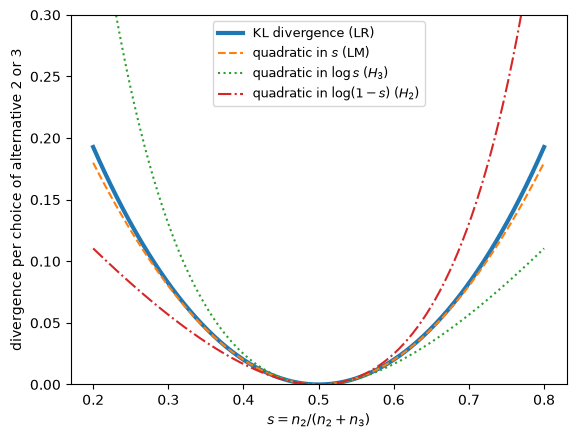
Fig. 25.1 KL divergence and its quadratic approximations#
The four statistics have the same asymptotic distribution under the null hypothesis and under local alternatives, but they differ in finite samples.
Hausman and McFadden tabulate exact rejection probabilities of these tests and of the Wald test of \(\lambda = 1\) in a nested logit model with parameter \(\lambda\).
Their alternatives are nested logit models with \(\lambda < 1\) that put alternatives 1 and 2 in one nest, so that \(p_2 < p_3\).
In their Tables III.2 and III.3, the Wald test and \(H_3\) are the most powerful, followed by the likelihood ratio and Lagrange multiplier tests, and \(H_2\) is the least powerful.
Their text names \(H_2\) in four places where the rows of their tables show \(H_3\), and \(H_3\) in one place where the tables show \(H_2\); the ranking they state on p. 1233, WALD > H3 > LR > LM > H2, agrees with the tables.
They report two “rather unexpected results”:
(i) The three tests which comprise the so-called holy trinity of asymptotic tests differ markedly in both of their operating characteristics even when their nominal size is the same. (ii) The Wald test and Hausman type test have approximately equal power. Next comes the LR test and the LM test. Both results may well arise because we are considering a nonlocal alternative hypothesis.
They add that “the samples may not be large enough for the reliable application of asymptotic theory.”
Exponential Family and Maximum Entropy compares quadratic approximations to KL divergence in natural and expectation coordinates for the Poisson family.
Exercise 25.1 computes exact sizes and powers.
25.5. Hansen and Sargent’s test of exogeneity#
Hansen and Sargent [1980] derive the cross-equation restrictions that a rational expectations model of a firm’s demand for labor imposes on the joint process of employment \(n_t\) and a vector \(x_t\) of variables that the firm takes as given.
The firm observes a shock \(a_t\) that the econometrician does not.
Given that employment does not Granger-cause \(x_t\), the vector \(x_t\) is strictly exogenous in the firm’s decision rule if and only if a vector \(v\) of regression coefficients is zero, which is equivalent to the requirement that the innovations in \(x_t\) be uncorrelated with the innovations in \(a_t\).
They write:
This latter test is similar in spirit to the test for exogeneity proposed by Wu (1973) in a classical simultaneous equations setting.
and add that their setting differs from Wu’s “in that we are allowing for serial correlation in disturbance terms and that we achieve parameter identification via non-linear cross-equation restrictions implied by the hypothesis of rational expectations.”
They propose to estimate the model twice by quasi-maximum likelihood, once with \(v\) free and once with \(v = 0\), and to compare the two likelihoods with a likelihood ratio statistic that is asymptotically \(\chi^2\) under the null hypothesis.
A second version tests \(v = 0\) with the estimated covariance matrix of \(\hat v\).
They also propose testing the cross-equation restrictions themselves by nesting the model within a more loosely specified model that does not impose them.
Stochastic Consumption, Risk Aversion, and the Temporal Behavior of Asset Returns applies such a test to the cross-equation restrictions that a consumption Euler equation imposes on a vector autoregression.
With the frequency-domain likelihood (24.5) of Approximation Errors in Time Series Models, each log likelihood is, up to a term that does not depend on the model, minus the sum over frequencies of the cross-entropies of \(N(0, I(\omega_j))\) relative to \(N(0, G(\omega_j, \delta))\).
Each likelihood ratio statistic is therefore a sum over frequencies.
Neither the unrestricted model nor the restricted model is an exponential family in general, and the cross-equation restrictions make the restricted model a curved subset of the unrestricted one.
The Pythagorean decomposition (23.3) therefore holds only to second order, which is the order that the asymptotic \(\chi^2\) distribution uses.
25.6. Comparing frequency bands#
We construct a Hausman test that compares the frequency-domain maximum likelihood estimator that uses all frequencies with the one that deletes the seasonal bands.
Approximation Errors in Time Series Models shows that deleting bands from Hansen and Sargent’s criterion, as in (24.6), projects the part of a process that lies outside the bands onto the part of the model that lies outside them.
When the model is correctly specified, the two estimators converge to the same parameter, and the estimator that uses all frequencies is efficient, so Hausman’s lemma applies.
When the model is misspecified at the seasonal frequencies, the two estimators converge to different projections.
In the seasonal example of Approximation Errors in Time Series Models, where the seasonal component has one quarter of the variance of the nonseasonal component, an AR(1) projection has \(\rho^* = 0.62\) with all frequencies and \(\rho^* = 0.87\) with bands of width \(\pi/8\) deleted.
With the 1 percent share used below, the solution to Exercise 25.2 computes \(0.885\) and \(0.899\).
For a Gaussian process and a correctly specified scalar model with spectral density \(g(\omega; \theta)\), \(\sqrt{T}\) times the error of the frequency-domain maximum likelihood estimator that uses the frequencies in a set \(K\) has asymptotic covariance matrix \(\mathcal{I}_K(\theta)^{-1}\), where
\(\mathcal{I}_K(\theta)\) is the curvature of a KL divergence, as in Exponential Family and Maximum Entropy: it is the Hessian at \(\theta' = \theta\) of the divergence rate (24.2), restricted to \(K\), of \(g(\cdot\,; \theta)\) from \(g(\cdot\,; \theta')\).
By (25.2), the difference between the band-deleted estimator and the full-band estimator has asymptotic covariance matrix \(\mathcal{I}_K(\theta)^{-1} - \mathcal{I}(\theta)^{-1}\), where \(\mathcal{I}\) uses all frequencies.
Deleting the bands is a garbling in the sense of Blackwell’s Theorem on Comparing Experiments, so \(\mathcal{I}_K(\theta) \preceq \mathcal{I}(\theta)\) by the Fisher-information form of the data processing inequality; inversion reverses the matrix order, so this covariance matrix is positive semidefinite.
We apply the test to a first-order autoregression with parameters \(\theta = (\rho, \sigma^2)\) fitted to \(T = 400\) quarterly observations, deleting bands of width \(\pi/8\) around \(\pi/2\) and \(\pi\), and we test only \(\rho\), using the \((1, 1)\) elements of these matrices.
Each estimator uses the Fourier frequencies \(\omega_j = 2\pi j / T\), \(j = 1, \ldots, T - 1\), omitting \(j = 0\) because the sample mean is removed, and we evaluate \(\mathcal{I}_K\) at the same frequencies, so that \(\frac{1}{4\pi} \int_K\) becomes \(\frac{1}{2T} \sum_{j \in K}\).
Omitting \(j = 0\) removes about 10 percent of the information about \(\rho\) at \(T = 400\), because the spectral density of \(x_t\) has a narrow peak at frequency zero; the \((1, 1)\) element of \(\mathcal{I}^{-1}\) is \(0.21\) rather than \(1 - \rho^2 = 0.19\).
In each sample we evaluate the two information matrices at the full-band estimate of \(\rho\).
Under the null hypothesis, the data come from \(x_t = 0.9 x_{t-1} + e_t\).
Under the alternatives, we add the seasonal component of Approximation Errors in Time Series Models, which we call \(w_t\) here because \(s\) denotes Hausman and McFadden’s share: \((1 + \varphi L + \varphi^2 L^2 + \varphi^3 L^3) w_t = \eta_t\), with \(\eta_t\) white noise and \(\varphi = 0.98\).
We scale \(\eta_t\) so that the variance of \(w_t\) is 0.5, 1, or 2 percent of the variance of \(x_t\).
T_obs, ρ_x, φ = 400, 0.9, 0.98
ω_T = 2 * np.pi * np.arange(1, T_obs) / T_obs
z_T = np.exp(-1j * ω_T)


def seasonal_keep(ω_set, Δ):
    """True outside bands of width Δ centered on π/2, π, and 3π/2."""
    def dist(c):
        return np.minimum(np.abs(ω_set - c), 2 * np.pi - np.abs(ω_set - c))
    inside = ((dist(np.pi / 2) < Δ / 2) | (dist(np.pi) < Δ / 2)
              | (dist(3 * np.pi / 2) < Δ / 2))
    return ~inside


keep_all = np.ones(T_obs - 1, bool)
keep_band = seasonal_keep(ω_T, np.pi / 8)
var_x = 1 / (1 - ρ_x**2)
ω_fine = 2 * np.pi * (np.arange(2**14) + 0.5) / 2**14
z_fine = np.exp(-1j * ω_fine)
var_w_unit = np.mean(1 / np.abs(1 + φ * z_fine + φ**2 * z_fine**2
                                + φ**3 * z_fine**3)**2)


def whittle_ar1(I, keep):
    """Frequency-domain ML estimate of ρ in an AR(1), over the frequencies in keep."""
    def criterion(ρ):
        a2 = np.abs(1 - ρ * z_T[keep])**2
        return np.log(np.mean(I[keep] * a2)) - np.mean(np.log(a2))
    return minimize_scalar(criterion, bounds=(-0.999, 0.999), method="bounded",
                           options={"xatol": 1e-8}).x


def ar1_information(ρ, keep):
    """(1/4π) ∫_K ∇log g ∇log g' dω at the Fourier frequencies, θ = (ρ, σ²), σ² = 1."""
    d = np.vstack([2 * (np.cos(ω_T) - ρ) / np.abs(1 - ρ * z_T)**2,
                   np.ones(T_obs - 1)])
    return 0.5 * (d[:, keep] @ d[:, keep].T) / T_obs


def band_test(share, seed, R=1000, burn=200):
    rng = np.random.default_rng(seed)
    stats, ρ_full, ρ_band = np.empty(R), np.empty(R), np.empty(R)
    scale = np.sqrt(share * var_x / var_w_unit)
    for r in range(R):
        x_ = lfilter([1], [1, -ρ_x], rng.normal(size=T_obs + burn))
        w_ = lfilter([1], [1, φ, φ**2, φ**3], rng.normal(size=T_obs + burn))
        y_ = (x_ + scale * w_)[burn:]
        I = np.abs(np.fft.fft(y_ - y_.mean()))[1:]**2 / T_obs
        ρ_full[r] = whittle_ar1(I, keep_all)
        ρ_band[r] = whittle_ar1(I, keep_band)
        V_full = np.linalg.inv(ar1_information(ρ_full[r], keep_all))[0, 0]
        V_band = np.linalg.inv(ar1_information(ρ_full[r], keep_band))[0, 0]
        stats[r] = T_obs * (ρ_band[r] - ρ_full[r])**2 / (V_band - V_full)
    return stats, ρ_full, ρ_band


crit_1 = chi2.ppf(0.95, 1)
stats, ρ_full, ρ_band = band_test(0.0, seed=2)
print(f"null: Var(band) = {ρ_band.var():.3e},  Var(full) + Var(band - full) = "
      f"{ρ_full.var() + (ρ_band - ρ_full).var():.3e}")
print(f"null: rejection frequency at 5%: {np.mean(stats > crit_1):.3f}")
V_full_0 = np.linalg.inv(ar1_information(ρ_x, keep_all))[0, 0]
V_band_0 = np.linalg.inv(ar1_information(ρ_x, keep_band))[0, 0]
print(f"V_band - V_full = {V_band_0 - V_full_0:.4f},  V_full = {V_full_0:.4f}")

# the same seed for every share gives common random numbers
simulated_power, band_draws = {}, {}
for share in (0.005, 0.01, 0.02):
    stats, ρ_full, ρ_band = band_test(share, seed=3)
    simulated_power[share] = np.mean(stats > crit_1)
    band_draws[share] = (ρ_full, ρ_band)
    print(f"seasonal variance {share:.3f} of Var(x): mean ρ_full = "
          f"{ρ_full.mean():.3f}, mean ρ_band = {ρ_band.mean():.3f}, "
          f"rejection frequency {simulated_power[share]:.3f}")
null: Var(band) = 5.724e-04,  Var(full) + Var(band - full) = 5.741e-04
null: rejection frequency at 5%: 0.046
V_band - V_full = 0.0048,  V_full = 0.2100
seasonal variance 0.005 of Var(x): mean ρ_full = 0.886, mean ρ_band = 0.893, rejection frequency 0.429
seasonal variance 0.010 of Var(x): mean ρ_full = 0.879, mean ρ_band = 0.892, rejection frequency 0.784
seasonal variance 0.020 of Var(x): mean ρ_full = 0.864, mean ρ_band = 0.891, rejection frequency 0.979
Under the null hypothesis, the simulated variances satisfy Hausman’s identity (25.2), and the test rejects at close to its nominal rate.
A seasonal component with one or two percent of the variance of \(x_t\) pulls the full-band estimate below the band-deleted estimate by enough for the test to reject in most samples; with half a percent, the test rejects in fewer than half of the samples.
The test is powerful because, for this model, deleting the seasonal bands costs little information about \(\rho\), whose information is concentrated at low frequencies: the \((1, 1)\) element of \(\mathcal{I}_K(\theta)^{-1} - \mathcal{I}(\theta)^{-1}\) is about 2 percent of the \((1, 1)\) element of \(\mathcal{I}(\theta)^{-1}\).
In the language of Garbling and the data processing inequality in Approximation Errors in Time Series Models, the numerator \(T(\hat\rho_{\text{band}} - \hat\rho_{\text{full}})^2\) of the statistic is \(T\) times the squared shift in the m-projection that deleting the bands causes, plus sampling noise, and the denominator measures the information that deleting them destroys, so the test has power when the shift is large relative to the lost information.
Exercise 25.2 computes the test’s asymptotic power from the distance between the two projections, and Turbulence, Earnings Instability, and Indirect Inference applies the same calculation to two explanations of rising earnings instability.
25.7. Concluding remarks#
Each specification test in this lecture compares two estimators whose probability limits coincide when the model is correctly specified, and each has no power against a misspecification that leaves the two probability limits equal.
With the variance held fixed, Wu’s statistic is the ratio of the squared lengths of the two legs of a right triangle whose Pythagorean theorem is the one for m-projections onto nested exponential families.
Hausman’s lemma is a Pythagorean theorem in the inner product defined by asymptotic covariances, and it is the local form of the Pythagorean theorem for m-projections when the inefficient estimator is the maximum likelihood estimator of a model that nests the null model.
In Hausman and McFadden’s three-choice example, the likelihood ratio, Lagrange multiplier, and Hausman statistics are \(2m\) times a KL divergence and its quadratic approximations in the coordinates \(s\), \(\log s\), and \(\log(1 - s)\).
In our example, with \(T = 400\) quarterly observations, a nonseasonal AR(1) with coefficient \(0.9\), and seasonal bands of width \(\pi/8\), the test that compares the estimators from all frequencies and from the frequencies outside the seasonal bands rejects in most samples when the seasonal component has at least 1 percent of the variance of the nonseasonal component.
Turbulence, Earnings Instability, and Indirect Inference compares the projections of a calibrated search model and of data onto an auxiliary statistical model, and Which Moments to Match? describes this comparison as indirect inference.
25.8. Exercises#
Exercise 25.1
Hausman and McFadden [1984] compute exact rejection probabilities of their tests by enumerating all possible outcomes of a sample of choices.
In the three-choice example, let the choice probabilities be \(p_1 = 0.5\) and \(p_2 = p_3 = 0.25\) under the null hypothesis, and let the sample size be \(N = 100\).
Conditional on \(m = n_2 + n_3\), what is the distribution of \(n_2\)? Use it to compute the exact probabilities with which the \(LR\), \(LM\), \(H_3\), and \(H_2\) statistics exceed the 5 percent critical value of the \(\chi^2_1\) distribution. Treat an infinite statistic as a rejection, and ignore the samples with \(m = 0\), which have probability \(0.5^{100}\).
Hausman and McFadden’s alternatives are nested logit models in which alternatives 1 and 2 share a nest. With parameter \(\lambda\) and \(\beta = \log 2\), let \(a = \beta/\lambda\), \(\Pi_1 = e^a/(e^a + 1)\), and \(p = (e^a + 1)^\lambda / (1 + (e^a + 1)^\lambda)\); then \(p_1 = \Pi_1 p\), \(p_2 = (1 - \Pi_1) p\), and \(p_3 = 1 - p\), and \(\lambda = 1\) gives the null probabilities. Repeat the calculation for \(\lambda = 0.8\) and compare your answers with their Table III.3.
Relate the differences among the four tests to Fig. 25.1.
Solution
Here is one solution.
Given \(m\), \(n_2\) is binomial with \(m\) trials and success probability \(p_2/(p_2 + p_3)\), and \(m\) is binomial with \(N\) trials and success probability \(p_2 + p_3\).
All four statistics depend only on \(m\) and \(n_2\).
def iia_statistics(n2, m):
    """LR, LM, H3, and H2 for an array of values of n2, given m = n2 + n3."""
    n3 = m - n2
    with np.errstate(divide="ignore", invalid="ignore"):
        LR = 2 * (np.where(n2 > 0, n2 * np.log(2 * n2 / m), 0)
                  + np.where(n3 > 0, n3 * np.log(2 * n3 / m), 0))
        H3 = np.where(n2 > 0, np.log(2 * n2 / m)**2 * m, np.inf)
        H2 = np.where(n3 > 0, np.log(2 * n3 / m)**2 * m, np.inf)
    LM = (n3 - n2)**2 / m
    return np.array([LR, LM, H3, H2])


def rejection_probabilities(p2, p3, N=100, level=0.05):
    crit = chi2.ppf(1 - level, 1)
    probs = np.zeros(4)
    for m in range(1, N + 1):
        n2 = np.arange(m + 1)
        weights = binom.pmf(m, N, p2 + p3) * binom.pmf(n2, m, p2 / (p2 + p3))
        probs += (iia_statistics(n2, m) > crit) @ weights
    return probs


def nested_logit(λ, β=np.log(2)):
    """Choice probabilities with alternatives 1 and 2 in one nest."""
    a = β / λ
    Π_1 = np.exp(a) / (np.exp(a) + 1)
    p = (np.exp(a) + 1)**λ / (1 + (np.exp(a) + 1)**λ)
    return Π_1 * p, (1 - Π_1) * p, 1 - p


for λ in (1.0, 0.8):
    p1, p2, p3 = nested_logit(λ)
    print(f"λ = {λ}: p = ({p1:.4f}, {p2:.4f}, {p3:.4f});  LR, LM, H3, H2 reject "
          f"with probabilities {np.round(rejection_probabilities(p2, p3), 4)}")
λ = 1.0: p = (0.5000, 0.2500, 0.2500);  LR, LM, H3, H2 reject with probabilities [0.0501 0.0494 0.055  0.055 ]
λ = 0.8: p = (0.5110, 0.2149, 0.2741);  LR, LM, H3, H2 reject with probabilities [0.1348 0.1336 0.1929 0.0839]
Under the null hypothesis, the exact sizes are \(0.050\) for the likelihood ratio test, \(0.049\) for the Lagrange multiplier test, and \(0.055\) for both Hausman tests; \(H_3\) and \(H_2\) have the same size because \(n_2\) and \(n_3\) have the same distribution under the null hypothesis.
Hausman and McFadden’s Table III.3 reports \(0.054\) for both Hausman tests at \(\lambda = 1\); exact enumeration gives \(0.055\), while their entries for \(\lambda < 1\) at the 5 percent level agree with exact enumeration to five digits.
With \(\lambda = 0.8\), the powers are \(0.135\), \(0.134\), \(0.193\), and \(0.084\), the values in Hausman and McFadden’s Table III.3.
The ranking follows from Fig. 25.1.
Under this alternative \(p_2 < p_3\), so most samples have \(s < \frac{1}{2}\).
For \(s < \frac{1}{2}\), the quadratic approximation in \(\log s\) lies above the KL divergence and the quadratic approximation in \(\log(1 - s)\) lies below it, so \(H_3\) is larger than \(LR\) and \(H_2\) is smaller; the quadratic approximation in \(\log(1 - s)\) also lies below the one in \(s\), so \(H_2\) is smaller than \(LM\).
In every sample \(LR \ge LM\), by Pinsker’s inequality \(D(\text{Bern}(s) \| \text{Bern}(\frac{1}{2})) \ge 2(s - \frac{1}{2})^2\): the quadratic approximation in \(s\) lies below the KL divergence.
Exercise 25.2
The power of the band comparison test depends on the distance between the two projections.
For seasonal variance shares \(0.005\), \(0.01\), and \(0.02\), compute the pseudo-true values \(\rho^*_{\text{full}}\) and \(\rho^*_{\text{band}}\), the AR(1) projections of the process \(y_t = x_t + w_t\) with all frequencies and with the seasonal bands deleted.
Compute the noncentrality parameter \(\nu = T (\rho^*_{\text{band}} - \rho^*_{\text{full}})^2 / (V_{\text{band}} - V_{\text{full}})\), with the variances evaluated at \(\rho^*_{\text{full}}\), and the asymptotic power \(P(\chi^2_1(\nu) > 3.84)\).
Compare the asymptotic powers with the simulated rejection frequencies, and explain the differences.
Solution
Here is one solution.
We compute the projections at the Fourier frequencies of a sample of size \(T\), using the spectral density of \(y_t\) in place of the periodogram.
def spectral_density_y(share):
    f_x = 1 / np.abs(1 - ρ_x * z_T)**2
    f_w = 1 / np.abs(1 + φ * z_T + φ**2 * z_T**2 + φ**3 * z_T**3)**2
    return f_x + share * var_x / var_w_unit * f_w


projections = {}
print("share   ρ*_full  ρ*_band     ν    asymptotic power   simulated power")
for share in (0.005, 0.01, 0.02):
    f_y = spectral_density_y(share)
    ρ_f, ρ_b = whittle_ar1(f_y, keep_all), whittle_ar1(f_y, keep_band)
    V_full = np.linalg.inv(ar1_information(ρ_f, keep_all))[0, 0]
    V_band = np.linalg.inv(ar1_information(ρ_f, keep_band))[0, 0]
    projections[share] = (ρ_f, ρ_b, V_full, V_band)
    nc = T_obs * (ρ_b - ρ_f)**2 / (V_band - V_full)
    power = ncx2.sf(crit_1, 1, nc)
    print(f"{share:5.3f} {ρ_f:8.3f} {ρ_b:8.3f} {nc:7.1f} {power:12.2f} "
          f"{simulated_power[share]:17.2f}")
share   ρ*_full  ρ*_band     ν    asymptotic power   simulated power
0.005    0.893    0.899     3.3         0.45              0.43
0.010    0.885    0.899    11.7         0.93              0.78
0.020    0.871    0.898    36.8         1.00              0.98
The asymptotic power rises with the squared distance between the two projections.
It is close to the simulated power at the smallest and largest shares and too high at the intermediate share.
The noncentral \(\chi^2\) approximation uses the variance of the difference between the two estimators under the null hypothesis.
The code below compares the simulated mean and standard deviation of that difference with the distance between the projections and with the standard deviation that the null-hypothesis variance implies.
print("share   mean difference   distance   SD   null SD   ratio   "
      "corr(ρ_full, difference)")
for share in (0.005, 0.01, 0.02):
    ρ_f, ρ_b, V_full, V_band = projections[share]
    ρ_full, ρ_band = band_draws[share]
    difference = ρ_band - ρ_full
    sd_null = np.sqrt((V_band - V_full) / T_obs)
    print(f"{share:5.3f} {difference.mean():13.4f} {ρ_b - ρ_f:12.4f} "
          f"{difference.std():8.4f} {sd_null:7.4f} {difference.std() / sd_null:7.2f} "
          f"{np.corrcoef(ρ_full, difference)[0, 1]:12.2f}")
share   mean difference   distance   SD   null SD   ratio   corr(ρ_full, difference)
0.005        0.0069       0.0068   0.0055  0.0037    1.48        -0.34
0.010        0.0137       0.0134   0.0079  0.0039    2.02        -0.50
0.020        0.0268       0.0266   0.0132  0.0044    3.01        -0.67
The mean of the simulated difference is close to the distance between the two projections at every share, but its standard deviation is about 1.5, 2, and 3 times the value that the null-hypothesis variance implies.
Under these alternatives the AR(1) model is misspecified and Hausman’s lemma no longer applies: the simulated correlation between \(\hat\rho_{\text{full}}\) and the difference is \(-0.34\), \(-0.50\), and \(-0.67\).
The full-band estimator uses the periodogram ordinates at the seasonal peaks, whose variances are proportional to the square of the spectral density there; the band-deleted estimator does not use them.
Those ordinates raise the variance of \(\hat\rho_{\text{full}}\) and of the difference, so \(V_{\text{band}} - V_{\text{full}}\) understates the variance of the difference.
The test statistic is then approximately a multiple of a noncentral \(\chi^2\) variable with a smaller noncentrality parameter than the approximation uses.
At the largest share both powers are near one, and at the smallest share the larger spread and the smaller noncentrality roughly offset.
At the intermediate share the smaller noncentrality dominates, and the approximation overstates the power.
Hausman and McFadden’s example shows the opposite error: “For \(\lambda\) less than .9 all the tests have greater exact power than the prediction of the asymptotic approximation.”
Once alternatives are nonlocal, the approximation can err in either direction.
Formula (24.13) of Approximation Errors in Time Series Models gives the asymptotic covariance matrix of each estimator under the alternative, which makes the explanation above quantitative.
The two estimators share the periodogram ordinates outside the bands, so the asymptotic covariance matrix between \(\sqrt{T}\) times the errors of the two estimators is \(\mathcal{H}^{-1} \mathcal{J}_{\text{cross}} \mathcal{H}_K^{-1}\), where
\(g_{\text{full}}\) and \(g_{\text{band}}\) are the spectral densities of the two projections, and \(\mathcal{H}\) and \(\mathcal{H}_K\) are the matrices \(\mathcal{H}_K\) of (24.13) for all frequencies and for the frequencies outside the bands, each evaluated at its own projection.
The code below computes from these matrices the ratio of the standard deviation of the difference to the null standard deviation, the correlation between \(\hat\rho_{\text{full}}\) and the difference, and the power of the test when the statistic is approximated by \(V_{\text{diff}} / (V_{\text{band}} - V_{\text{full}})\) times a noncentral \(\chi^2_1\) variable with noncentrality \(T (\rho^*_{\text{band}} - \rho^*_{\text{full}})^2 / V_{\text{diff}}\), where \(V_{\text{diff}}\) is the asymptotic variance of the difference under the alternative.
def ar1_derivatives(ρ, σ2):
    """∇ log g and ∇² log g at the Fourier frequencies, θ = (ρ, σ²)."""
    d1 = np.vstack([2 * (np.cos(ω_T) - ρ) / np.abs(1 - ρ * z_T)**2,
                    np.ones(T_obs - 1) / σ2])
    d2 = np.zeros((2, 2, T_obs - 1))
    d2[0, 0] = 2 * np.real(z_T**2 / (1 - ρ * z_T)**2)
    d2[1, 1] = -1 / σ2**2
    return d1, d2


def projection_parts(f, keep):
    """AR(1) projection over keep, the inverse of H, ∇ log g, and f/g on keep."""
    ρ = whittle_ar1(f, keep)
    σ2 = np.mean((f * np.abs(1 - ρ * z_T)**2)[keep])
    d1, d2 = ar1_derivatives(ρ, σ2)
    r = np.where(keep, f * np.abs(1 - ρ * z_T)**2 / σ2, 0.0)
    H = 0.5 * ((d1 * r) @ d1.T
               + (d2 * np.where(keep, 1 - r, 0.0)).sum(axis=2)) / T_obs
    return ρ, np.linalg.inv(H), d1, r


def score_covariance(d_a, r_a, d_b, r_b):
    return 0.5 * ((d_a * r_a * r_b) @ d_b.T) / T_obs


print("share   SD ratio   corr(ρ_full, difference)   power   simulated power")
for share in (0.005, 0.01, 0.02):
    f_y = spectral_density_y(share)
    ρ_f, H_f, d_f, r_f = projection_parts(f_y, keep_all)
    ρ_b, H_b, d_b, r_b = projection_parts(f_y, keep_band)
    V_f = (H_f @ score_covariance(d_f, r_f, d_f, r_f) @ H_f)[0, 0]
    V_b = (H_b @ score_covariance(d_b, r_b, d_b, r_b) @ H_b)[0, 0]
    C_fb = (H_f @ score_covariance(d_f, r_f, d_b, r_b) @ H_b)[0, 0]
    V_diff = V_f + V_b - 2 * C_fb
    _, _, V_full, V_band = projections[share]
    V_null = V_band - V_full
    power = ncx2.sf(crit_1 * V_null / V_diff, 1, T_obs * (ρ_b - ρ_f)**2 / V_diff)
    print(f"{share:5.3f} {np.sqrt(V_diff / V_null):9.2f} "
          f"{(C_fb - V_f) / np.sqrt(V_f * V_diff):19.2f} {power:15.2f} "
          f"{simulated_power[share]:12.2f}")
share   SD ratio   corr(ρ_full, difference)   power   simulated power
0.005      1.42               -0.34            0.47         0.43
0.010      1.96               -0.51            0.77         0.78
0.020      2.96               -0.68            0.92         0.98
The covariance matrices under the alternative give ratios of \(1.42\), \(1.96\), and \(2.96\) and correlations of \(-0.34\), \(-0.51\), and \(-0.68\), close to the simulated \(1.48\), \(2.02\), and \(3.01\) and \(-0.34\), \(-0.50\), and \(-0.67\).
The power approximation that uses them gives \(0.47\), \(0.77\), and \(0.92\), against simulated powers of \(0.43\), \(0.78\), and \(0.98\): it corrects the error at the intermediate share, is slightly farther from the simulation than the null approximation at the smallest share, and understates the power at the largest share.