68. The Income Fluctuation Problem II: Optimistic Policy Iteration#
GPU
This lecture was built using a machine with access to a GPU — although it will also run without one.
Google Colab has a free tier with GPUs that you can access as follows:
Click on the “play” icon top right
Select Colab
Set the runtime environment to include a GPU
68.1. Overview#
In The Income Fluctuation Problem I: Discretization and VFI we studied the income fluctuation problem and solved it using value function iteration (VFI).
In this lecture we’ll solve the same problem using optimistic policy iteration (OPI), which is very general, typically faster than VFI and only slightly more complex.
OPI combines elements of both value function iteration and policy iteration.
A detailed discussion of the algorithm can be found in DP1.
Here our aim is to implement OPI and test whether or not it yields significant speed improvements over standard VFI for the income fluctuation problem.
In addition to Anaconda, this lecture will need the following libraries:
!pip install quantecon jax
We will use the following imports:
import quantecon as qe
import jax
import jax.numpy as jnp
import matplotlib.pyplot as plt
from typing import NamedTuple
from time import time
68.2. Model and Primitives#
The model and parameters are the same as in The Income Fluctuation Problem I: Discretization and VFI.
We repeat the key elements here for convenience.
The household’s problem is to maximize
subject to
where \(u(c) = c^{1-\gamma}/(1-\gamma)\).
Here’s the model structure:
class Model(NamedTuple):
    β: float              # Discount factor
    R: float              # Gross interest rate
    γ: float              # CRRA parameter
    a_grid: jnp.ndarray   # Asset grid
    y_grid: jnp.ndarray   # Income grid
    Q: jnp.ndarray        # Markov matrix for income


def create_consumption_model(
        R=1.01,                    # Gross interest rate
        β=0.98,                    # Discount factor
        γ=2,                       # CRRA parameter
        a_min=0.01,                # Min assets
        a_max=10.0,                # Max assets
        a_size=150,                # Grid size
        ρ=0.9, ν=0.1, y_size=100   # Income parameters
    ):
    """
    Creates an instance of the consumption-savings model.

    """
    a_grid = jnp.linspace(a_min, a_max, a_size)
    mc = qe.tauchen(n=y_size, rho=ρ, sigma=ν)
    y_grid, Q = jnp.exp(mc.state_values), jax.device_put(mc.P)
    return Model(β, R, γ, a_grid, y_grid, Q)
68.3. Operators and Policies#
We repeat some functions from The Income Fluctuation Problem I: Discretization and VFI.
Here is the right hand side of the Bellman equation:
def B(v, model, i, j, ip):
    """
    The right-hand side of the Bellman equation before maximization, which takes
    the form

        B(a, y, a′) = u(Ra + y - a′) + β Σ_y′ v(a′, y′) Q(y, y′)

    The indices are (i, j, ip) -> (a, y, a′).
    """
    β, R, γ, a_grid, y_grid, Q = model
    a, y, ap  = a_grid[i], y_grid[j], a_grid[ip]
    c = R * a + y - ap
    EV = jnp.sum(v[ip, :] * Q[j, :])
    return jnp.where(c > 0, c**(1-γ)/(1-γ) + β * EV, -jnp.inf)
Now we successively apply vmap to vectorize over all indices:
B_1    = jax.vmap(B,   in_axes=(None, None, None, None, 0))
B_2    = jax.vmap(B_1, in_axes=(None, None, None, 0,    None))
B_vmap = jax.vmap(B_2, in_axes=(None, None, 0,    None, None))
Here’s the Bellman operator:
def T(v, model):
    "The Bellman operator."
    a_indices = jnp.arange(len(model.a_grid))
    y_indices = jnp.arange(len(model.y_grid))
    B_values = B_vmap(v, model, a_indices, y_indices, a_indices)
    return jnp.max(B_values, axis=-1)
Here’s the function that computes a \(v\)-greedy policy:
def get_greedy(v, model):
    "Computes a v-greedy policy, returned as a set of indices."
    a_indices = jnp.arange(len(model.a_grid))
    y_indices = jnp.arange(len(model.y_grid))
    B_values = B_vmap(v, model, a_indices, y_indices, a_indices)
    return jnp.argmax(B_values, axis=-1)
Now we define the policy operator \(T_\sigma\), which is the Bellman operator with policy \(\sigma\) fixed.
For a given policy \(\sigma\), the policy operator is defined by
def T_σ(v, σ, model, i, j):
    """
    The σ-policy operator for indices (i, j) -> (a, y).
    """
    β, R, γ, a_grid, y_grid, Q = model

    # Get values at current state
    a, y = a_grid[i], y_grid[j]
    # Get policy choice
    ap = a_grid[σ[i, j]]

    # Compute current reward
    c = R * a + y - ap
    r = jnp.where(c > 0, c**(1-γ)/(1-γ), -jnp.inf)

    # Compute expected value
    EV = jnp.sum(v[σ[i, j], :] * Q[j, :])

    return r + β * EV
Apply vmap to vectorize:
T_σ_1    = jax.vmap(T_σ,   in_axes=(None, None, None, None, 0))
T_σ_vmap = jax.vmap(T_σ_1, in_axes=(None, None, None, 0,    None))

def T_σ_vec(v, σ, model):
    """Vectorized version of T_σ."""
    a_size, y_size = len(model.a_grid), len(model.y_grid)
    a_indices = jnp.arange(a_size)
    y_indices = jnp.arange(y_size)
    return T_σ_vmap(v, σ, model, a_indices, y_indices)
Now we need a function to apply the policy operator m times:
def iterate_policy_operator(σ, v, m, model):
    """
    Apply the policy operator T_σ exactly m times to v.
    """
    def update(i, v):
        return T_σ_vec(v, σ, model)

    v = jax.lax.fori_loop(0, m, update, v)
    return v
68.4. Value Function Iteration#
For comparison, here’s VFI from The Income Fluctuation Problem I: Discretization and VFI:
@jax.jit
def value_function_iteration(model, tol=1e-5, max_iter=10_000):
    """
    Implements VFI using successive approximation.
    """
    def body_fun(k_v_err):
        k, v, error = k_v_err
        v_new = T(v, model)
        error = jnp.max(jnp.abs(v_new - v))
        return k + 1, v_new, error

    def cond_fun(k_v_err):
        k, v, error = k_v_err
        return jnp.logical_and(error > tol, k < max_iter)

    v_init = jnp.zeros((len(model.a_grid), len(model.y_grid)))
    k, v_star, error = jax.lax.while_loop(cond_fun, body_fun,
                                          (1, v_init, tol + 1))
    return v_star, get_greedy(v_star, model)
68.5. Optimistic Policy Iteration#
Now we implement OPI.
The algorithm alternates between
Performing \(m\) policy operator iterations to update the value function
Computing a new greedy policy based on the updated value function
@jax.jit
def optimistic_policy_iteration(model, m=10, tol=1e-5, max_iter=10_000):
    """
    Implements optimistic policy iteration with step size m.

    Parameters:
    -----------
    model : Model
        The consumption-savings model
    m : int
        Number of policy operator iterations per step
    tol : float
        Tolerance for convergence
    max_iter : int
        Maximum number of iterations
    """
    v_init = jnp.zeros((len(model.a_grid), len(model.y_grid)))

    def condition_function(inputs):
        i, v, error = inputs
        return jnp.logical_and(error > tol, i < max_iter)

    def update(inputs):
        i, v, error = inputs
        last_v = v
        σ = get_greedy(v, model)
        v = iterate_policy_operator(σ, v, m, model)
        error = jnp.max(jnp.abs(v - last_v))
        i += 1
        return i, v, error

    num_iter, v, error = jax.lax.while_loop(condition_function,
                                            update,
                                            (0, v_init, tol + 1))

    return v, get_greedy(v, model)
68.6. Timing Comparison#
Let’s create a model and compare the performance of VFI and OPI.
model = create_consumption_model()
First, let’s time VFI:
print("Starting VFI.")
start = time()
v_star_vfi, σ_star_vfi = value_function_iteration(model)
v_star_vfi.block_until_ready()
vfi_time_with_compile = time() - start
print(f"VFI completed in {vfi_time_with_compile:.2f} seconds.")
Starting VFI.
VFI completed in 0.52 seconds.
Run it again to eliminate compile time:
start = time()
v_star_vfi, σ_star_vfi = value_function_iteration(model)
v_star_vfi.block_until_ready()
vfi_time = time() - start
print(f"VFI completed in {vfi_time:.2f} seconds.")
VFI completed in 0.11 seconds.
Now let’s time OPI with different values of m:
print("Starting OPI with m=50.")
start = time()
v_star_opi, σ_star_opi = optimistic_policy_iteration(model, m=50)
v_star_opi.block_until_ready()
opi_time_with_compile = time() - start
print(f"OPI completed in {opi_time_with_compile:.2f} seconds.")
Starting OPI with m=50.
OPI completed in 0.35 seconds.
Run it again:
start = time()
v_star_opi, σ_star_opi = optimistic_policy_iteration(model, m=50)
v_star_opi.block_until_ready()
opi_time = time() - start
print(f"OPI completed in {opi_time:.2f} seconds.")
OPI completed in 0.04 seconds.
Check that we get the same result:
print(f"Values match: {jnp.allclose(v_star_vfi, v_star_opi)}")
Values match: True
The value functions match, confirming both algorithms converge to the same solution.
Let’s visually compare the asset dynamics under both policies:
fig, axes = plt.subplots(1, 2, figsize=(12, 5))

# VFI policy
for j, label in zip([0, -1], ['low income', 'high income']):
    a_next_vfi = model.a_grid[σ_star_vfi[:, j]]
    axes[0].plot(model.a_grid, a_next_vfi, label=label)
axes[0].plot(model.a_grid, model.a_grid, 'k--', linewidth=0.5, alpha=0.5)
axes[0].set(xlabel='current assets', ylabel='next period assets', title='VFI')
axes[0].legend()

# OPI policy
for j, label in zip([0, -1], ['low income', 'high income']):
    a_next_opi = model.a_grid[σ_star_opi[:, j]]
    axes[1].plot(model.a_grid, a_next_opi, label=label)
axes[1].plot(model.a_grid, model.a_grid, 'k--', linewidth=0.5, alpha=0.5)
axes[1].set(xlabel='current assets', ylabel='next period assets', title='OPI')
axes[1].legend()

plt.tight_layout()
plt.show()
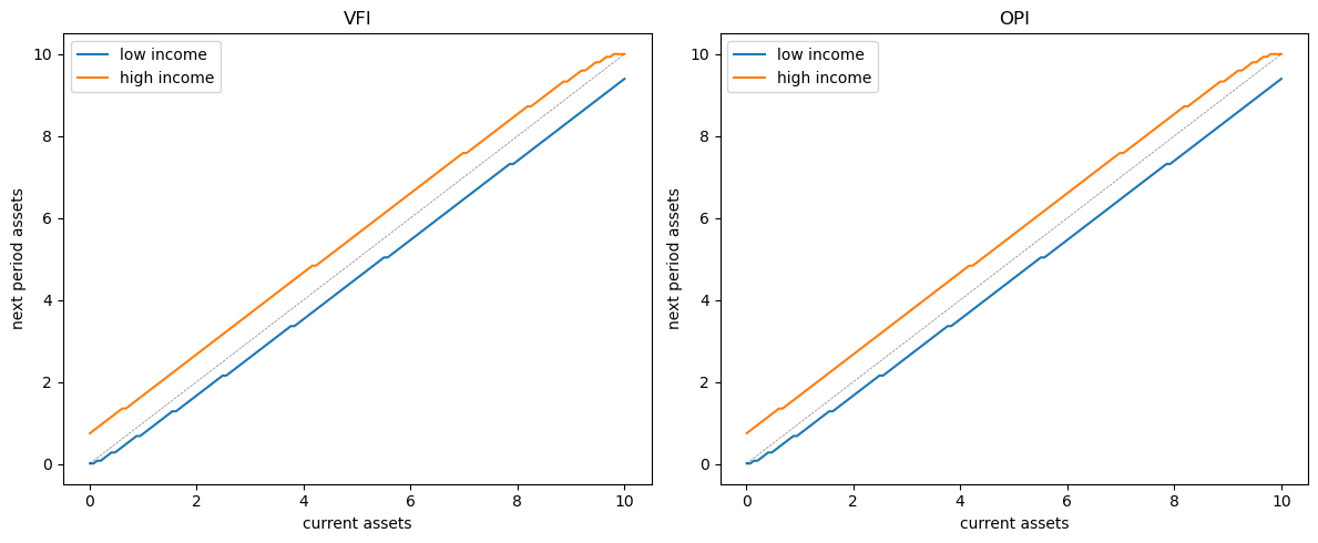
The policies are visually indistinguishable, confirming both methods produce the same solution.
Here’s the speedup:
print(f"Speedup factor: {vfi_time / opi_time:.2f}")
Speedup factor: 2.87
Let’s try different values of m to see how it affects performance:
m_vals = [1, 5, 10, 25, 50, 100, 200, 400]
opi_times = []

for m in m_vals:
    start = time()
    v_star, σ_star = optimistic_policy_iteration(model, m=m)
    v_star.block_until_ready()
    elapsed = time() - start
    opi_times.append(elapsed)
    print(f"OPI with m={m:3d} completed in {elapsed:.2f} seconds.")
OPI with m=  1 completed in 0.12 seconds.
OPI with m=  5 completed in 0.05 seconds.
OPI with m= 10 completed in 0.04 seconds.
OPI with m= 25 completed in 0.04 seconds.
OPI with m= 50 completed in 0.03 seconds.
OPI with m=100 completed in 0.04 seconds.
OPI with m=200 completed in 0.07 seconds.
OPI with m=400 completed in 0.14 seconds.
Plot the results:
fig, ax = plt.subplots()
ax.plot(m_vals, opi_times, 'o-', label='OPI')
ax.axhline(vfi_time, linestyle='--', color='red', label='VFI')
ax.set_xlabel('m (policy steps per iteration)')
ax.set_ylabel('time (seconds)')
ax.legend()
ax.set_title('OPI execution time vs step size m')
plt.show()
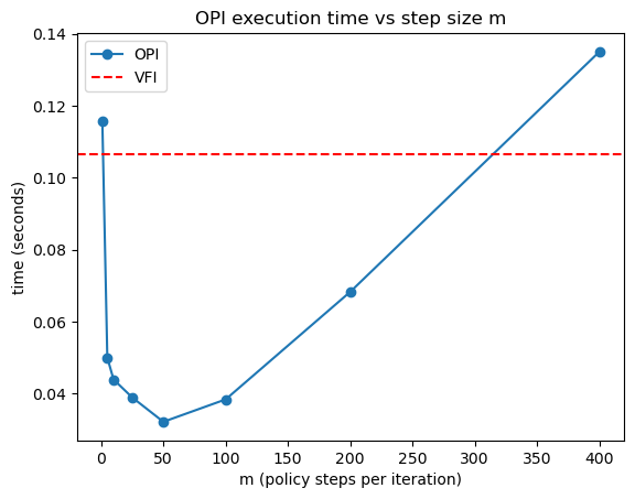
Here’s a summary of the results
OPI outperforms VFI for a large range of \(m\) values.
For very large \(m\), OPI performance begins to degrade as we spend too much time iterating the policy operator.
68.7. Exercises#
Exercise 68.1
The speed gains achieved by OPI are quite robust to parameter changes.
Confirm this by experimenting with different parameter values for the income process (\(\rho\) and \(\nu\)).
Measure how they affect the relative performance of VFI vs OPI.
Try:
\(\rho \in \{0.8, 0.9, 0.95\}\)
\(\nu \in \{0.05, 0.1, 0.2\}\)
For each combination, compute the speedup factor (VFI time / OPI time) and report your findings.
Solution
Here’s one solution:
ρ_vals = [0.8, 0.9, 0.95]
ν_vals = [0.05, 0.1, 0.2]

results = []

for ρ in ρ_vals:
    for ν in ν_vals:
        print(f"\nTesting ρ={ρ}, ν={ν}")

        # Create model
        model = create_consumption_model(ρ=ρ, ν=ν)

        # Time VFI
        start = time()
        v_vfi, σ_vfi = value_function_iteration(model)
        v_vfi.block_until_ready()
        vfi_t = time() - start

        # Time OPI
        start = time()
        v_opi, σ_opi = optimistic_policy_iteration(model, m=10)
        v_opi.block_until_ready()
        opi_t = time() - start

        speedup = vfi_t / opi_t
        results.append((ρ, ν, speedup))
        print(f"  VFI: {vfi_t:.2f}s, OPI: {opi_t:.2f}s, Speedup: {speedup:.2f}x")

# Print summary
print("\nSummary of speedup factors:")
for ρ, ν, speedup in results:
    print(f"ρ={ρ}, ν={ν}: {speedup:.2f}x")
Testing ρ=0.8, ν=0.05
  VFI: 0.06s, OPI: 0.04s, Speedup: 1.64x

Testing ρ=0.8, ν=0.1
  VFI: 0.06s, OPI: 0.03s, Speedup: 1.82x

Testing ρ=0.8, ν=0.2
  VFI: 0.06s, OPI: 0.03s, Speedup: 1.74x

Testing ρ=0.9, ν=0.05
  VFI: 0.06s, OPI: 0.03s, Speedup: 1.77x

Testing ρ=0.9, ν=0.1
  VFI: 0.06s, OPI: 0.04s, Speedup: 1.68x

Testing ρ=0.9, ν=0.2
  VFI: 0.06s, OPI: 0.04s, Speedup: 1.78x

Testing ρ=0.95, ν=0.05
  VFI: 0.06s, OPI: 0.04s, Speedup: 1.73x

Testing ρ=0.95, ν=0.1
  VFI: 0.06s, OPI: 0.04s, Speedup: 1.73x

Testing ρ=0.95, ν=0.2
  VFI: 0.07s, OPI: 0.04s, Speedup: 1.84x

Summary of speedup factors:
ρ=0.8, ν=0.05: 1.64x
ρ=0.8, ν=0.1: 1.82x
ρ=0.8, ν=0.2: 1.74x
ρ=0.9, ν=0.05: 1.77x
ρ=0.9, ν=0.1: 1.68x
ρ=0.9, ν=0.2: 1.78x
ρ=0.95, ν=0.05: 1.73x
ρ=0.95, ν=0.1: 1.73x
ρ=0.95, ν=0.2: 1.84x