26. A Problem that Stumped Milton Friedman #

(and that Abraham Wald solved by inventing sequential analysis)

Contents

A Problem that Stumped Milton Friedman

26.1. Overview #

This is the first of two lectures about a statistical decision problem that a US Navy Captain presented to Milton Friedman and W. Allen Wallis during World War II when they were analysts at the U.S. Government’s Statistical Research Group at Columbia University.

This problem led Abraham Wald [Wald, 1947] to formulate sequential analysis, an approach to statistical decision problems that is intimately related to dynamic programming.

In the spirit of this earlier lecture, the present lecture and its sequel approach the problem from two distinct points of view, one frequentist, the other Bayesian.

In this lecture, we describe Wald’s formulation of the problem from the perspective of a statistician working within the Neyman-Pearson tradition of a frequentist statistician who thinks about testing hypotheses and consequently use laws of large numbers to investigate limiting properties of particular statistics under a given hypothesis, i.e., a vector of parameters that pins down a particular member of a manifold of statistical models that interest the statistician.

From this lecture on frequentist and bayesian statistics, please remember that a frequentist statistician routinely calculates functions of sequences of random variables, conditioning on a vector of parameters.

In this related lecture we’ll discuss another formulation that adopts the perspective of a Bayesian statistician who views parameters as random variables that are jointly distributed with observable variables that he is concerned about.

Because we are taking a frequentist perspective that is concerned about relative frequencies conditioned on alternative parameter values, i.e., alternative hypotheses, key ideas in this lecture

Type I and type II statistical errors
- a type I error occurs when you reject a null hypothesis that is true
- a type II error occurs when you accept a null hypothesis that is false
The power of a frequentist statistical test
The size of a frequentist statistical test
The critical region of a statistical test
A uniformly most powerful test
The role of a Law of Large Numbers (LLN) in interpreting power and size of a frequentist statistical test
Abraham Wald’s sequential probability ratio test

We’ll begin with some imports:

import numpy as np
import matplotlib.pyplot as plt
from numba import njit, prange, vectorize, jit
from numba.experimental import jitclass
from math import gamma
from scipy.integrate import quad
from scipy.stats import beta
from collections import namedtuple
import pandas as pd
import scipy as sp

This lecture uses ideas studied in the lecture on likelihood ratio processes and the lecture on Bayesian learning.

26.2. Source of the Problem #

On pages 137-139 of his 1998 book Two Lucky People with Rose Friedman [Friedman and Friedman, 1998], Milton Friedman described a problem presented to him and Allen Wallis during World War II, when they worked at the US Government’s Statistical Research Group at Columbia University.

Note

See pages 25 and 26 of Allen Wallis’s 1980 article [Wallis, 1980] about the Statistical Research Group at Columbia University during World War II for his account of the episode and for important contributions that Harold Hotelling made to formulating the problem. Also see chapter 5 of Jennifer Burns’ book about Milton Friedman [Burns, 2023].

Let’s listen to Milton Friedman tell us what happened

In order to understand the story, it is necessary to have an idea of a simple statistical problem, and of the standard procedure for dealing with it. The actual problem out of which sequential analysis grew will serve. The Navy has two alternative designs (say A and B) for a projectile. It wants to determine which is superior. To do so it undertakes a series of paired firings. On each round, it assigns the value 1 or 0 to A accordingly as its performance is superior or inferior to that of B and conversely 0 or 1 to B. The Navy asks the statistician how to conduct the test and how to analyze the results.

The standard statistical answer was to specify a number of firings (say 1,000) and a pair of percentages (e.g., 53% and 47%) and tell the client that if A receives a 1 in more than 53% of the firings, it can be regarded as superior; if it receives a 1 in fewer than 47%, B can be regarded as superior; if the percentage is between 47% and 53%, neither can be so regarded.

When Allen Wallis was discussing such a problem with (Navy) Captain Garret L. Schuyler, the captain objected that such a test, to quote from Allen’s account, may prove wasteful. If a wise and seasoned ordnance officer like Schuyler were on the premises, he would see after the first few thousand or even few hundred [rounds] that the experiment need not be completed either because the new method is obviously inferior or because it is obviously superior beyond what was hoped for $\ldots$.

Friedman and Wallis worked on the problem for a while but didn’t completely solve it.

Realizing that, they told Abraham Wald about the problem.

That set Wald on a path that led him to create Sequential Analysis [Wald, 1947].

26.3. Neyman-Pearson formulation #

It is useful to begin by describing the theory underlying the test that the U.S. Navy told Captain G. S. Schuyler to use.

Captain Schuyler’s doubts motivated him to tell Milton Friedman and Allen Wallis his conjecture that superior practical procedures existed.

Evidently, the Navy had told Captain Schuyler to use what was then a state-of-the-art Neyman-Pearson hypothesis test.

We’ll rely on Abraham Wald’s [Wald, 1947] elegant summary of Neyman-Pearson theory.

Watch for these features of the setup:

the assumption of a fixed sample size $n$
the application of laws of large numbers, conditioned on alternative probability models, to interpret probabilities $\alpha$ and $\beta$ of the type I and type II errors defined in the Neyman-Pearson theory

In chapter 1 of Sequential Analysis [Wald, 1947] Abraham Wald summarizes the Neyman-Pearson approach to hypothesis testing.

Wald frames the problem as making a decision about a probability distribution that is partially known.

(You have to assume that something is already known in order to state a well-posed problem – usually, something means a lot)

By limiting what is unknown, Wald uses the following simple structure to illustrate the main ideas:

A decision-maker wants to decide which of two distributions $f_0$, $f_1$ govern an IID random variable $z$.
The null hypothesis $H_0$ is the statement that $f_0$ governs the data.
The alternative hypothesis $H_1$ is the statement that $f_1$ governs the data.
The problem is to devise and analyze a test of hypothesis $H_0$ against the alternative hypothesis $H_1$ on the basis of a sample of a fixed number $n$ independent observations $z_1, z_2, \ldots, z_n$ of the random variable $z$.

To quote Abraham Wald,

A test procedure leading to the acceptance or rejection of the [null] hypothesis in question is simply a rule specifying, for each possible sample of size $n$, whether the [null] hypothesis should be accepted or rejected on the basis of the sample. This may also be expressed as follows: A test procedure is simply a subdivision of the totality of all possible samples of size $n$ into two mutually exclusive parts, say part 1 and part 2, together with the application of the rule that the [null] hypothesis be accepted if the observed sample is contained in part 2. Part 1 is also called the critical region. Since part 2 is the totality of all samples of size $n$ which are not included in part 1, part 2 is uniquely determined by part 1. Thus, choosing a test procedure is equivalent to determining a critical region.

Let’s listen to Wald longer:

As a basis for choosing among critical regions the following considerations have been advanced by Neyman and Pearson: In accepting or rejecting $H_0$ we may commit errors of two kinds. We commit an error of the first kind if we reject $H_0$ when it is true; we commit an error of the second kind if we accept $H_0$ when $H_1$ is true. After a particular critical region $W$ has been chosen, the probability of committing an error of the first kind, as well as the probability of committing an error of the second kind is uniquely determined. The probability of committing an error of the first kind is equal to the probability, determined by the assumption that $H_0$ is true, that the observed sample will be included in the critical region $W$. The probability of committing an error of the second kind is equal to the probability, determined on the assumption that $H_1$ is true, that the probability will fall outside the critical region $W$. For any given critical region $W$ we shall denote the probability of an error of the first kind by $\alpha$ and the probability of an error of the second kind by $\beta$.

Let’s listen carefully to how Wald applies law of large numbers to interpret $\alpha$ and $\beta$:

The probabilities $\alpha$ and $\beta$ have the following important practical interpretation: Suppose that we draw a large number of samples of size $n$. Let $M$ be the number of such samples drawn. Suppose that for each of these $M$ samples we reject $H_0$ if the sample is included in $W$ and accept $H_0$ if the sample lies outside $W$. In this way we make $M$ statements of rejection or acceptance. Some of these statements will in general be wrong. If $H_0$ is true and if $M$ is large, the probability is nearly $1$ (i.e., it is practically certain) that the proportion of wrong statements (i.e., the number of wrong statements divided by $M$) will be approximately $\alpha$. If $H_1$ is true, the probability is nearly $1$ that the proportion of wrong statements will be approximately $\beta$. Thus, we can say that in the long run [ here Wald applies law of large numbers by driving $M \rightarrow \infty$ (our comment, not Wald’s) ] the proportion of wrong statements will be $\alpha$ if $H_0$ is true and $\beta$ if $H_1$ is true.

The quantity $\alpha$ is called the size of the critical region, and the quantity $1-\beta$ is called the power of the critical region.

Wald notes that

one critical region $W$ is more desirable than another if it has smaller values of $\alpha$ and $\beta$. Although either $\alpha$ or $\beta$ can be made arbitrarily small by a proper choice of the critical region $W$, it is impossible to make both $\alpha$ and $\beta$ arbitrarily small for a fixed value of $n$, i.e., a fixed sample size.

Wald summarizes Neyman and Pearson’s setup as follows:

Neyman and Pearson show that a region consisting of all samples $(z_1, z_2, \ldots, z_n)$ which satisfy the inequality

\[ \frac{ f_1(z_1) \cdots f_1(z_n)}{f_0(z_1) \cdots f_0(z_n)} \geq k \]

is a most powerful critical region for testing the hypothesis $H_0$ against the alternative hypothesis $H_1$. The term $k$ on the right side is a constant chosen so that the region will have the required size $\alpha$.

Wald goes on to discuss Neyman and Pearson’s concept of uniformly most powerful test.

Here is how Wald introduces the notion of a sequential test

A rule is given for making one of the following three decisions at any stage of the experiment (at the $m$ th trial for each integral value of $m$): (1) to accept the hypothesis $H$, (2) to reject the hypothesis $H$, (3) to continue the experiment by making an additional observation. Thus, such a test procedure is carried out sequentially. On the basis of the first observation, one of the aforementioned decision is made. If the first or second decision is made, the process is terminated. If the third decision is made, a second trial is performed. Again, on the basis of the first two observations, one of the three decision is made. If the third decision is made, a third trial is performed, and so on. The process is continued until either the first or the second decisions is made. The number $n$ of observations required by such a test procedure is a random variable, since the value of $n$ depends on the outcome of the observations.

26.4. Wald’s sequential formulation #

By way of contrast to Neyman and Pearson’s formulation of the problem, in Wald’s formulation

The sample size $n$ is not fixed but rather a random variable.
Two parameters $A$ and $B$ that are related to but distinct from Neyman and Pearson’s $\alpha$ and $\beta$; $A$ and $B$ characterize cut-off rules that Wald uses to determine the random variable $n$ as a function of random outcomes.

Here is how Wald sets up the problem.

A decision-maker can observe a sequence of draws of a random variable $z$.

He (or she) wants to know which of two probability distributions $f_0$ or $f_1$ governs $z$.

We use beta distributions as examples.

We will also work with Jensen-Shannon divergence introduced in Statistical Divergence Measures.

@vectorize
def p(x, a, b):
    """Beta distribution density function."""
    r = gamma(a + b) / (gamma(a) * gamma(b))
    return r * x** (a-1) * (1 - x) ** (b-1)

def create_beta_density(a, b):
    """Create a beta density function with specified parameters."""
    return jit(lambda x: p(x, a, b))

def compute_KL(f, g):
    """Compute KL divergence KL(f, g)"""
    integrand = lambda w: f(w) * np.log(f(w) / g(w))
    val, _ = quad(integrand, 1e-5, 1-1e-5)
    return val

def compute_JS(f, g):
    """Compute Jensen-Shannon divergence"""
    def m(w):
        return 0.5 * (f(w) + g(w))
    
    js_div = 0.5 * compute_KL(f, m) + 0.5 * compute_KL(g, m)
    return js_div

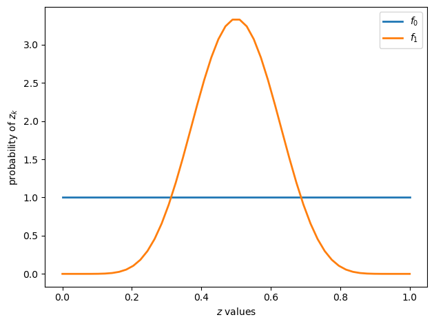
The next figure shows two beta distributions

f0 = create_beta_density(1, 1)
f1 = create_beta_density(9, 9)
grid = np.linspace(0, 1, 50)

fig, ax = plt.subplots()
ax.plot(grid, f0(grid), lw=2, label="$f_0$")
ax.plot(grid, f1(grid), lw=2, label="$f_1$")
ax.legend()
ax.set(xlabel="$z$ values", ylabel="probability of $z_k$")
plt.tight_layout()
plt.show()

_images/069cb35421161f4c4895e2ca18df0619baa841e37da25c54252a43ffba4bfc49.png

Conditional on knowing that successive observations are drawn from distribution $f_0$, the sequence of random variables is independently and identically distributed (IID).

Conditional on knowing that successive observations are drawn from distribution $f_1$, the sequence of random variables is also independently and identically distributed (IID).

But the observer does not know which of the two distributions generated the sequence.

For reasons explained in Exchangeability and Bayesian Updating, this means that the observer thinks that the sequence is not IID.

Consequently, the observer has something to learn, namely, whether the observations are drawn from $f_0$ or from $f_1$.

The decision maker wants to decide which of the two distributions is generating outcomes.

26.4.1. Type I and type II errors#

If we regard $f=f_0$ as a null hypothesis and $f=f_1$ as an alternative hypothesis, then

a type I error is an incorrect rejection of a true null hypothesis (a “false positive”)
a type II error is a failure to reject a false null hypothesis (a “false negative”)

To repeat ourselves

$\alpha$ is the probability of a type I error
$\beta$ is the probability of a type II error

26.4.2. Choices#

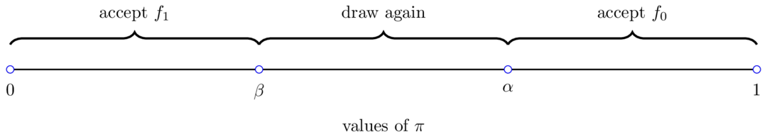
After observing $z_k, z_{k-1}, \ldots, z_1$, the decision-maker chooses among three distinct actions:

He decides that $f = f_0$ and draws no more $z$’s
He decides that $f = f_1$ and draws no more $z$’s
He postpones deciding and instead chooses to draw $z_{k+1}$

Wald defines

$p_{0m} = f_0(z_1) \cdots f_0(z_m)$
$p_{1m} = f_1(z_1) \cdots f_1(z_m)$
$L_{m} = \frac{p_{1m}}{p_{0m}}$

Here $\{L_m\}_{m=0}^\infty$ is a likelihood ratio process.

Wald’s sequential decision rule is parameterized by real numbers $B < A$.

For a given pair $A, B$, the decision rule is

\[\begin{split} \begin{aligned} \textrm { accept } f=f_1 \textrm{ if } L_m \geq A \\ \textrm { accept } f=f_0 \textrm{ if } L_m \leq B \\ \textrm { draw another } z \textrm{ if } B < L_m < A \end{aligned} \end{split}\]

The following figure illustrates aspects of Wald’s procedure.

26.5. Links between $A,B$ and $\alpha, \beta$#

In chapter 3 of Sequential Analysis [Wald, 1947] Wald establishes the inequalities

\[\begin{split} \begin{aligned} \frac{\alpha}{1 -\beta} & \leq \frac{1}{A} \\ \frac{\beta}{1 - \alpha} & \leq B \end{aligned} \end{split}\]

His analysis of these inequalities leads Wald to recommend the following approximations as rules for setting $A$ and $B$ that come close to attaining a decision maker’s target values for probabilities $\alpha$ of a type I and $\beta$ of a type II error:

(26.1)#\[\begin{split} \begin{aligned} A \approx a(\alpha,\beta) & \equiv \frac{1-\beta}{\alpha} \\ B \approx b(\alpha,\beta) & \equiv \frac{\beta}{1-\alpha} \end{aligned} \end{split}\]

For small values of $\alpha$ and $\beta$, Wald shows that approximation (26.1) provides a good way to set $A$ and $B$.

In particular, Wald constructs a mathematical argument that leads him to conclude that the use of approximation (26.1) rather than the true functions $A (\alpha, \beta), B(\alpha,\beta)$ for setting $A$ and $B$

$\ldots$ cannot result in any appreciable increase in the value of either $\alpha$ or $\beta$. In other words, for all practical purposes the test corresponding to $A = a(\alpha, \beta), B = b(\alpha,\beta)$ provides as least the same protection against wrong decisions as the test corresponding to $A = A(\alpha, \beta)$ and $B = b(\alpha, \beta)$.

Thus, the only disadvantage that may arise from using $ a(\alpha, \beta), b(\alpha,\beta)$ instead of $ A(\alpha, \beta), B(\alpha,\beta)$, respectively, is that it may result in an appreciable increase in the number of observations required by the test.

We’ll write some Python code to help us illustrate Wald’s claims about how $\alpha$ and $\beta$ are related to the parameters $A$ and $B$ that characterize his sequential probability ratio test.

26.6. Simulations #

We experiment with different distributions $f_0$ and $f_1$ to examine how Wald’s test performs under various conditions.

Our goal in conducting these simulations is to understand trade-offs between decision speed and accuracy associated with Wald’s sequential probability ratio test.

Specifically, we will watch how:

The decision thresholds $A$ and $B$ (or equivalently the target error rates $\alpha$ and $\beta$) affect the average stopping time
The discrepancy between distributions $f_0$ and $f_1$ affects average stopping times

We will focus on the case where $f_0$ and $f_1$ are beta distributions since it is easy to control the overlapping regions of the two densities by adjusting their shape parameters.

First, we define a namedtuple to store all the parameters we need for our simulation studies.

We also compute Wald’s recommended thresholds $A$ and $B$ based on the target type I and type II errors $\alpha$ and $\beta$

SPRTParams = namedtuple('SPRTParams', 
                ['α', 'β',  # Target type I and type II errors
                'a0', 'b0', # Shape parameters for f_0
                'a1', 'b1', # Shape parameters for f_1
                'N',        # Number of simulations
                'seed'])

@njit
def compute_wald_thresholds(α, β):
    """Compute Wald's recommended thresholds."""
    A = (1 - β) / α
    B = β / (1 - α)
    return A, B, np.log(A), np.log(B)

Now we can run the simulation following Wald’s recommendation.

We’ll compare the log-likelihood ratio to logarithms of the thresholds $\log(A)$ and $\log(B)$.

The following algorithm underlies our simulations.

Compute thresholds $A = \frac{1-\beta}{\alpha}$, $B = \frac{\beta}{1-\alpha}$ and work with $\log A$, $\log B$.
Given true distribution (either $f_0$ or $f_1$):
- Initialize log-likelihood ratio $\log L_0 = 0$
- Repeat:
  - Draw observation $z$ from the true distribution
  - Update: $\log L_{n+1} \leftarrow \log L_n + (\log f_1(z) - \log f_0(z))$
  - If $\log L_{n+1} \geq \log A$: stop, reject $H_0$
  - If $\log L_{n+1} \leq \log B$: stop, accept $H_0$
Repeat step 2 for $N$ replications with $N/2$ replications for each distribution, compute the empirical type I error $\hat{\alpha}$ and type II error $\hat{\beta}$ with

\[ \hat{\alpha} = \frac{\text{$\#$ of times reject } H_0 \text{ when } f_0 \text{ is true}}{\text{$\#$ of replications with } f_0 \text{ true}} \]

\[ \hat{\beta} = \frac{\text{$\#$ of times accept } H_0 \text{ when } f_1 \text{ is true}}{\text{$\#$ of replications with } f_1 \text{ true}} \]

@njit
def sprt_single_run(a0, b0, a1, b1, logA, logB, true_f0, seed):
    """Run a single SPRT until a decision is reached."""
    log_L = 0.0
    n = 0
    np.random.seed(seed)
    
    while True:
        z = np.random.beta(a0, b0) if true_f0 else np.random.beta(a1, b1)
        n += 1
        
        # Update log-likelihood ratio
        log_L += np.log(p(z, a1, b1)) - np.log(p(z, a0, b0))
        
        # Check stopping conditions
        if log_L >= logA:
            return n, False  # Reject H0
        elif log_L <= logB:
            return n, True   # Accept H0

@njit(parallel=True)
def run_sprt_simulation(a0, b0, a1, b1, α, β, N, seed):
    """SPRT simulation."""
    A, B, logA, logB = compute_wald_thresholds(α, β)
    
    stopping_times = np.zeros(N, dtype=np.int64)
    decisions_h0 = np.zeros(N, dtype=np.bool_)
    truth_h0 = np.zeros(N, dtype=np.bool_)
    
    for i in prange(N):
        true_f0 = (i % 2 == 0)
        truth_h0[i] = true_f0
        
        n, accept_f0 = sprt_single_run(
                        a0, b0, a1, b1, 
                        logA, logB, 
                        true_f0, seed + i)
        stopping_times[i] = n
        decisions_h0[i] = accept_f0
    
    return stopping_times, decisions_h0, truth_h0

def run_sprt(params):
    """Run SPRT simulations with given parameters."""
    stopping_times, decisions_h0, truth_h0 = run_sprt_simulation(
        params.a0, params.b0, params.a1, params.b1, 
        params.α, params.β, params.N, params.seed
    )
    
    # Calculate error rates
    truth_h0_bool = truth_h0.astype(bool)
    decisions_h0_bool = decisions_h0.astype(bool)
    
    type_I = np.sum(truth_h0_bool & ~decisions_h0_bool) \
            / np.sum(truth_h0_bool)
    type_II = np.sum(~truth_h0_bool & decisions_h0_bool) \
            / np.sum(~truth_h0_bool)
    
    return {
        'stopping_times': stopping_times,
        'decisions_h0': decisions_h0_bool,
        'truth_h0': truth_h0_bool,
        'type_I': type_I,
        'type_II': type_II
    }

# Run simulation
params = SPRTParams(α=0.05, β=0.10, a0=2, b0=5, a1=5, b1=2, N=20000, seed=1)
results = run_sprt(params)

print(f"Average stopping time: {results['stopping_times'].mean():.2f}")
print(f"Empirical type I  error: {results['type_I']:.3f} (target = {params.α})")
print(f"Empirical type II error: {results['type_II']:.3f} (target = {params.β})")

Average stopping time: 1.59
Empirical type I  error: 0.012 (target = 0.05)
Empirical type II error: 0.022 (target = 0.1)

As anticipated in the passage above in which Wald discussed the quality of $a(\alpha, \beta), b(\alpha, \beta)$ given in approximation (26.1), we find that the algorithm actually gives lower type I and type II error rates than the target values.

Note

For recent work on the quality of approximation (26.1), see, e.g., [Fischer and Ramdas, 2024].

The following code creates a few graphs that illustrate the results of our simulation.

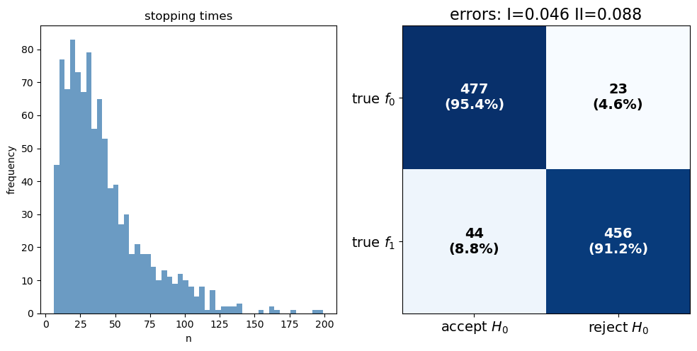
Let’s plot the results of our simulation

plot_sprt_results(results, params)

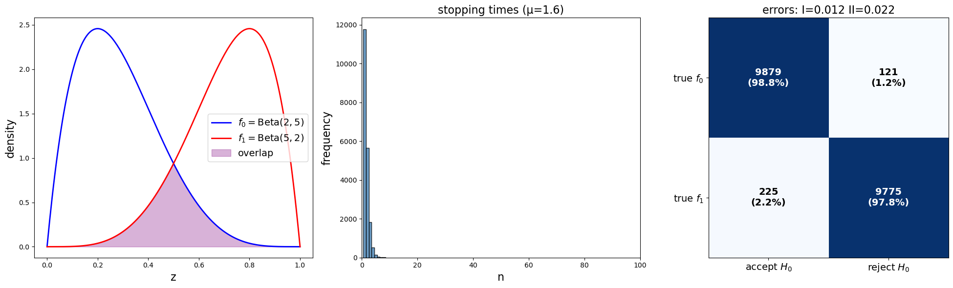
_images/d03e7b87bb06b9bd21bf0354cc012d85acda25d5b4182a86cfdf1030da469d9e.png

In this example, the stopping time stays below 10.

We can construct a $2 \times 2$ “confusion matrix” whose diagonal elements count the number of times that Wald’s decision rule correctly accepts and rejects the null hypothesis.

print("Confusion Matrix data:")
print(f"Type I error: {results['type_I']:.3f}")
print(f"Type II error: {results['type_II']:.3f}")

Confusion Matrix data:
Type I error: 0.012
Type II error: 0.022

Next we use our code to study three different $f_0, f_1$ pairs having different discrepancies between distributions.

We plot the same three graphs we used above for each pair of distributions

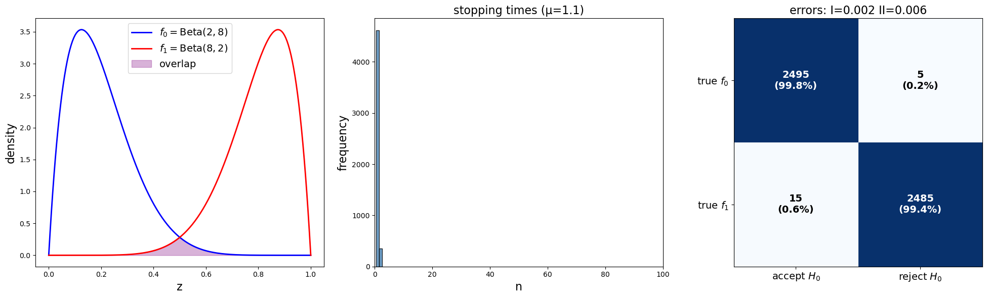
params_1 = SPRTParams(α=0.05, β=0.10, a0=2, b0=8, a1=8, b1=2, N=5000, seed=42)
results_1 = run_sprt(params_1)

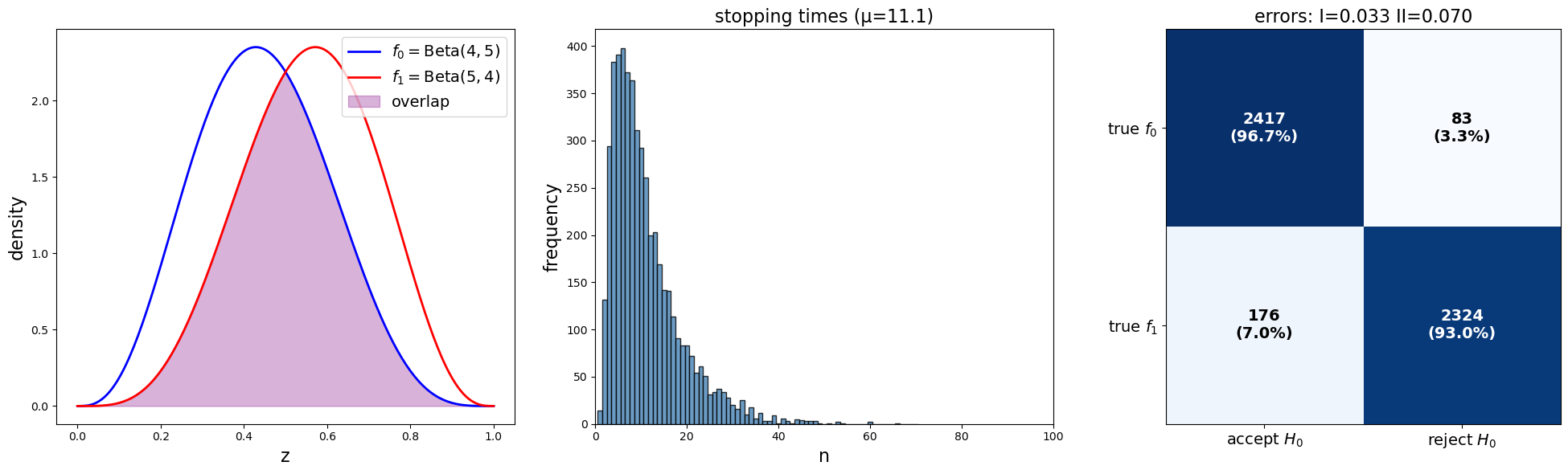
params_2 = SPRTParams(α=0.05, β=0.10, a0=4, b0=5, a1=5, b1=4, N=5000, seed=42)
results_2 = run_sprt(params_2)

params_3 = SPRTParams(α=0.05, β=0.10, a0=0.5, b0=0.4, a1=0.4, 
                      b1=0.5, N=5000, seed=42)
results_3 = run_sprt(params_3)

plot_sprt_results(results_1, params_1)

_images/8303cb2c05fbdce8145d2412c1624fbb1b2355d58d75aa21f54b5c35cf89e6cb.png

plot_sprt_results(results_2, params_2)

_images/c10afcef6e898989b031126482a03baa7f1979c01fe2e4e8f4d0dd35b1e21740.png

plot_sprt_results(results_3, params_3)

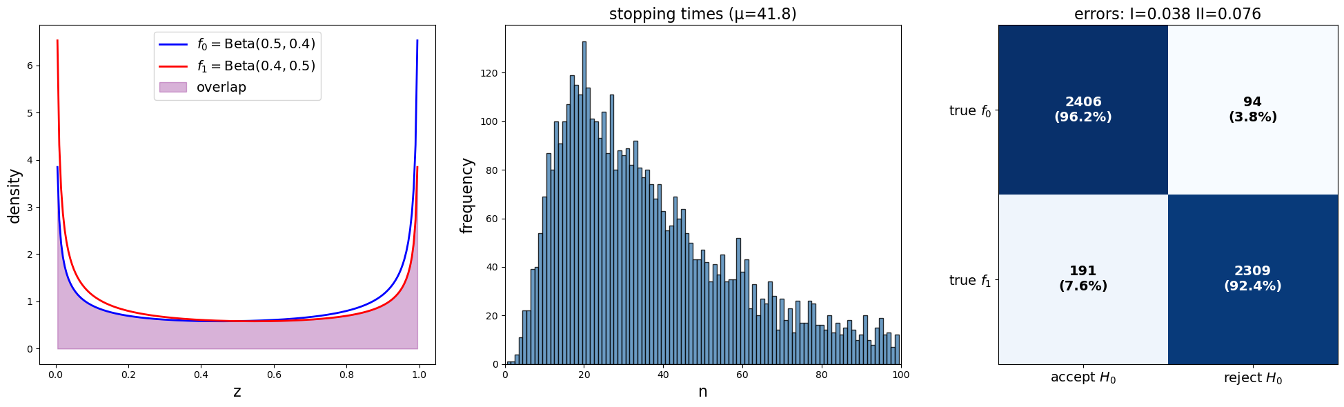
_images/dbd026a405576a8441e24540cd5e81b9c620b714aee72e10d202059d407c48db.png

Notice that the stopping times are less when the two distributions are farther apart.

This makes sense.

When two distributions are “far apart”, it should not take too long to decide which one is generating the data.

When two distributions are “close”, it should takes longer to decide which one is generating the data.

It is tempting to link this pattern to our discussion of Kullback–Leibler divergence in Likelihood Ratio Processes.

While, KL divergence is larger when two distributions differ more, KL divergence is not symmetric, meaning that the KL divergence of distribution $f$ from distribution $g$ is not necessarily equal to the KL divergence of $g$ from $f$.

If we want a symmetric measure of divergence that actually a metric, we can instead use Jensen-Shannon distance.

That is what we shall do now.

We shall compute Jensen-Shannon distance and plot it against the average stopping times.

def js_dist(a0, b0, a1, b1):
    """Jensen–Shannon distance"""
    f0 = create_beta_density(a0, b0)
    f1 = create_beta_density(a1, b1)

    # Mixture
    m = lambda w: 0.5*(f0(w) + f1(w))
    return np.sqrt(0.5*compute_KL(m, f0) + 0.5*compute_KL(m, f1))
    
def generate_β_pairs(N=100, T=10.0, d_min=0.5, d_max=9.5):
    ds = np.linspace(d_min, d_max, N)
    a0 = (T - ds) / 2
    b0 = (T + ds) / 2
    return list(zip(a0, b0, b0, a0))

param_comb = generate_β_pairs()

# Run simulations for each parameter combination
js_dists = []
mean_stopping_times = []
param_list = []

for a0, b0, a1, b1 in param_comb:
    # Compute KL divergence
    js_div = js_dist(a1, b1, a0, b0)
    
    # Run SPRT simulation with a fixed set of parameters d d
    params = SPRTParams(α=0.05, β=0.10, a0=a0, b0=b0, 
                        a1=a1, b1=b1, N=5000, seed=42)
    results = run_sprt(params)
    
    js_dists.append(js_div)
    mean_stopping_times.append(results['stopping_times'].mean())
    param_list.append((a0, b0, a1, b1))

# Create the plot
fig, ax = plt.subplots()

scatter = ax.scatter(js_dists, mean_stopping_times, 
                    s=80, alpha=0.7, linewidth=0.5)

ax.set_xlabel('Jensen–Shannon distance', fontsize=14)
ax.set_ylabel('mean stopping time', fontsize=14)

plt.tight_layout()
plt.show()

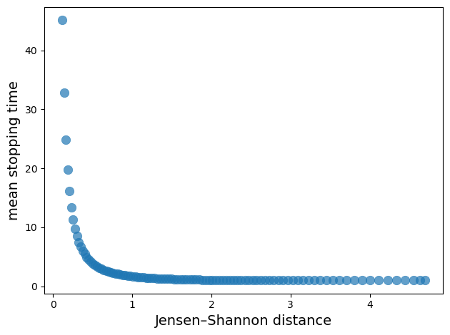
_images/cd4729272309ab702f8269f190dd361feb657085c52ab30cc2aeffef055cba95.png

The plot demonstrates a clear negative correlation between relative entropy and mean stopping time.

As Jensen-Shannon divergence increases (distributions become more separated), the mean stopping time decreases exponentially.

Below are sampled examples from the experiments we have above

def plot_beta_distributions_grid(param_list, js_dists, mean_stopping_times, 
                                selected_indices=None):
    """Plot grid of beta distributions with JS distance and stopping times."""
    if selected_indices is None:
        selected_indices = [0, len(param_list)//6, len(param_list)//3, 
                          len(param_list)//2, 2*len(param_list)//3, -1]
    
    fig, axes = plt.subplots(2, 3, figsize=(15, 8))
    z_grid = np.linspace(0, 1, 200)
    
    for i, idx in enumerate(selected_indices):
        row, col = i // 3, i % 3
        a0, b0, a1, b1 = param_list[idx]
        
        f0 = create_beta_density(a0, b0)
        f1 = create_beta_density(a1, b1)
        
        axes[row, col].plot(z_grid, f0(z_grid), 'b-', lw=2, label='$f_0$')
        axes[row, col].plot(z_grid, f1(z_grid), 'r-', lw=2, label='$f_1$')
        axes[row, col].fill_between(z_grid, 0, 
                                  np.minimum(f0(z_grid), f1(z_grid)), 
                                  alpha=0.3, color='purple')
        
        axes[row, col].set_title(f'JS dist: {js_dists[idx]:.3f}'
                               f'\nMean time: {mean_stopping_times[idx]:.1f}', 
                               fontsize=12)
        axes[row, col].set_xlabel('z', fontsize=10)
        if i == 0:
            axes[row, col].set_ylabel('density', fontsize=10)
            axes[row, col].legend(fontsize=10)

    plt.tight_layout()
    plt.show()

plot_beta_distributions_grid(param_list, js_dists, mean_stopping_times)

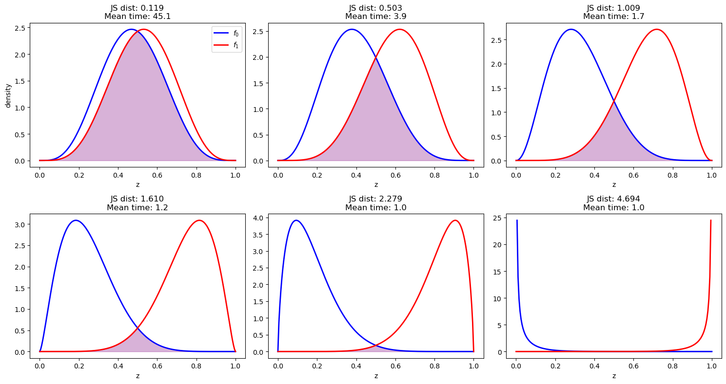
_images/c2bb5b4876bfbcd81bda74b1a5c8660124756963c353448297f2b94847d44855.png

Again, we find that the stopping time is shorter when the distributions are more separated, as measured by Jensen-Shannon distance.

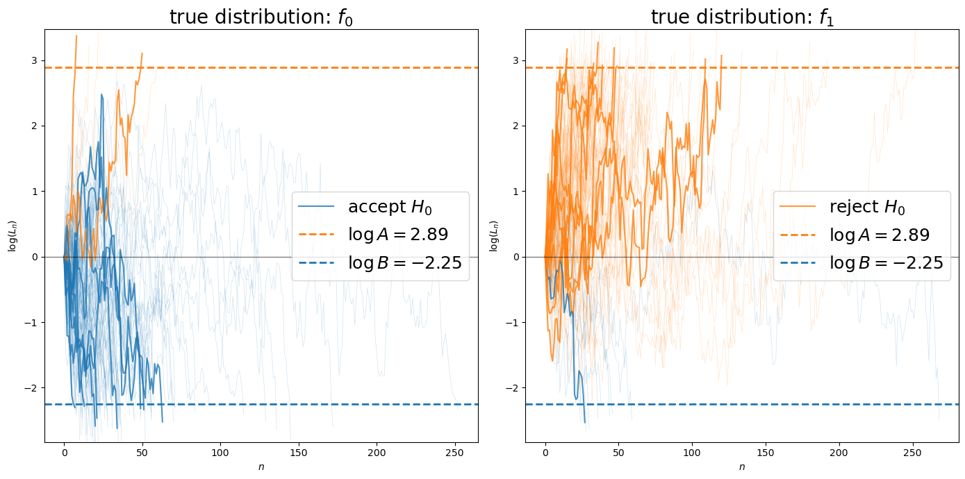
Let’s visualize individual likelihood ratio processes to see how they evolve toward the decision boundaries.

def plot_likelihood_paths(params, n_highlight=10, n_background=200):
    """visualize likelihood ratio paths."""
    A, B, logA, logB = compute_wald_thresholds(params.α, params.β)
    f0, f1 = map(lambda ab: create_beta_density(*ab),
             [(params.a0, params.b0), 
              (params.a1, params.b1)])
    
    fig, axes = plt.subplots(1, 2, figsize=(14, 7))
    
    for dist_idx, (true_f0, ax, title) in enumerate([
        (True, axes[0], 'true distribution: $f_0$'),
        (False, axes[1], 'true distribution: $f_1$')
    ]):
        rng = np.random.default_rng(seed=42 + dist_idx)
        paths_data = []
        
        # Generate paths
        for path in range(n_background + n_highlight):
            log_L_path, log_L, n = [0.0], 0.0, 0
            
            while True:
                z = rng.beta(params.a0, params.b0) if true_f0 \
                    else rng.beta(params.a1, params.b1)
                n += 1
                log_L += np.log(f1(z)) - np.log(f0(z))
                log_L_path.append(log_L)
                
                if log_L >= logA or log_L <= logB:
                    paths_data.append((log_L_path, n, log_L >= logA))
                    break
        
        # Plot background paths
        for path, _, decision in paths_data[:n_background]:
            ax.plot(range(len(path)), path, color='C1' if decision else 'C0', 
                   alpha=0.2, linewidth=0.5)
        
        # Plot highlighted paths with labels
        for i, (path, _, decision) in enumerate(paths_data[n_background:]):
            ax.plot(range(len(path)), path, color='C1' if decision else 'C0', 
                   alpha=0.8, linewidth=1.5,
                   label='reject $H_0$' if decision and i == 0 else (
                         'accept $H_0$' if not decision and i == 0 else ''))
        
        # Add threshold lines and formatting
        ax.axhline(y=logA, color='C1', linestyle='--', linewidth=2, 
                  label=f'$\\log A = {logA:.2f}$')
        ax.axhline(y=logB, color='C0', linestyle='--', linewidth=2, 
                  label=f'$\\log B = {logB:.2f}$')
        ax.axhline(y=0, color='black', linestyle='-', alpha=0.5, linewidth=1)
        
        ax.set_xlabel(r'$n$') 
        ax.set_ylabel(r'$\log(L_n)$')
        ax.set_title(title, fontsize=20)
        ax.legend(fontsize=18, loc='center right')
        
        y_margin = max(abs(logA), abs(logB)) * 0.2
        ax.set_ylim(logB - y_margin, logA + y_margin)
    
    plt.tight_layout()
    plt.show()

plot_likelihood_paths(params_3, n_highlight=10, n_background=100)

_images/f078311a426cab6ea90fc2f5e86e4cce3489dd15d97ea9eadc88d49ba17079de.png

Next, let’s adjust the decision thresholds $A$ and $B$ and examine how the mean stopping time and the type I and type II error rates change.

In the code below, we adjust Wald’s rule by adjusting the thresholds $A$ and $B$ using factors $A_f$ and $B_f$.

@njit(parallel=True)  
def run_adjusted_thresholds(a0, b0, a1, b1, α, β, N, seed, A_f, B_f):
    """SPRT simulation with adjusted thresholds."""
    
    # Calculate original thresholds  
    A_original = (1 - β) / α
    B_original = β / (1 - α)
    
    # Apply adjustment factors
    A_adj = A_original * A_f
    B_adj = B_original * B_f
    logA = np.log(A_adj)
    logB = np.log(B_adj)
    
    # Pre-allocate arrays
    stopping_times = np.zeros(N, dtype=np.int64)
    decisions_h0 = np.zeros(N, dtype=np.bool_)
    truth_h0 = np.zeros(N, dtype=np.bool_)
    
    # Run simulations in parallel
    for i in prange(N):
        true_f0 = (i % 2 == 0)
        truth_h0[i] = true_f0
        
        n, accept_f0 = sprt_single_run(a0, b0, a1, b1, 
                        logA, logB, true_f0, seed + i)
        stopping_times[i] = n
        decisions_h0[i] = accept_f0
    
    return stopping_times, decisions_h0, truth_h0, A_adj, B_adj

def run_adjusted(params, A_f=1.0, B_f=1.0):
    """Wrapper to run SPRT with adjusted A and B thresholds."""
    
    stopping_times, decisions_h0, truth_h0, A_adj, B_adj = run_adjusted_thresholds(
        params.a0, params.b0, params.a1, params.b1, 
        params.α, params.β, params.N, params.seed, A_f, B_f
    )
    truth_h0_bool = truth_h0.astype(bool)
    decisions_h0_bool = decisions_h0.astype(bool)
    
    # Calculate error rates
    type_I = np.sum(truth_h0_bool 
                    & ~decisions_h0_bool) / np.sum(truth_h0_bool)
    type_II = np.sum(~truth_h0_bool 
                    & decisions_h0_bool) / np.sum(~truth_h0_bool)
    
    return {
        'stopping_times': stopping_times,
        'type_I': type_I,
        'type_II': type_II,
        'A_used': A_adj,
        'B_used': B_adj
    }

adjustments = [
    (5.0, 0.5), 
    (1.0, 1.0),    
    (0.3, 3.0),    
    (0.2, 5.0),    
    (0.15, 7.0),   
]

results_table = []
for A_f, B_f in adjustments:
    result = run_adjusted(params_2, A_f, B_f)
    results_table.append([
        A_f, B_f, 
        f"{result['stopping_times'].mean():.1f}",
        f"{result['type_I']:.3f}",
        f"{result['type_II']:.3f}"
    ])

df = pd.DataFrame(results_table, 
                 columns=["A_f", "B_f", "mean stop time", 
                          "Type I error", "Type II error"])
df = df.set_index(["A_f", "B_f"])
df

		mean stop time	Type I error	Type II error
A_f	B_f
5.00	0.5	16.1	0.006	0.036
1.00	1.0	11.1	0.033	0.070
0.30	3.0	5.5	0.086	0.195
0.20	5.0	3.4	0.120	0.304
0.15	7.0	2.2	0.146	0.410

Let’s pause and think about the table more carefully by referring back to (26.1).

Recall that $A = \frac{1-\beta}{\alpha}$ and $B = \frac{\beta}{1-\alpha}$.

When we multiply $A$ by a factor less than 1 (making $A$ smaller), we are effectively making it easier to reject the null hypothesis $H_0$.

This increases the probability of Type I errors.

When we multiply $B$ by a factor greater than 1 (making $B$ larger), we are making it easier to accept the null hypothesis $H_0$.

This increases the probability of Type II errors.

The table confirms this intuition: as $A$ decreases and $B$ increases from their optimal Wald values, both Type I and Type II error rates increase, while the mean stopping time decreases.

26.8. Exercises #

In the two exercises below, please try to rewrite the entire SPRT suite in this lecture.

Exercise 26.1

In the first exercise, we apply the sequential probability ratio test to distinguish two models generated by 3-state Markov chains

(For a review on likelihood ratio processes for Markov chains, see this section.)

Consider distinguishing between two 3-state Markov chain models using Wald’s sequential probability ratio test.

You have competing hypotheses about the transition probabilities:

$H_0$: The chain follows transition matrix $P^{(0)}$
$H_1$: The chain follows transition matrix $P^{(1)}$

Given transition matrices:

\[\begin{split} P^{(0)} = \begin{bmatrix} 0.7 & 0.2 & 0.1 \\ 0.3 & 0.5 & 0.2 \\ 0.1 & 0.3 & 0.6 \end{bmatrix}, \quad P^{(1)} = \begin{bmatrix} 0.5 & 0.3 & 0.2 \\ 0.2 & 0.6 & 0.2 \\ 0.2 & 0.2 & 0.6 \end{bmatrix} \end{split}\]

For a sequence of observations $(x_0, x_1, \ldots, x_t)$, the likelihood ratio is:

\[ \Lambda_t = \frac{\pi_{x_0}^{(1)}}{\pi_{x_0}^{(0)}} \prod_{s=1}^t \frac{P_{x_{s-1},x_s}^{(1)}}{P_{x_{s-1},x_s}^{(0)}} \]

where $\pi^{(i)}$ is the stationary distribution under hypothesis $i$.

Tasks:

Implement the likelihood ratio computation for Markov chains
Implement Wald’s sequential test with Type I error $\alpha = 0.05$ and Type II error $\beta = 0.10$
Run 1000 simulations under each hypothesis and compute empirical error rates
Analyze the distribution of stopping times

The test stops when:

$\Lambda_t \geq A = \frac{1-\beta}{\alpha} = 18$: Reject $H_0$
$\Lambda_t \leq B = \frac{\beta}{1-\alpha} = 0.105$: Accept $H_0$

Solution to Exercise 26.1

Below is one solution to the exercise.

In the lecture, we write the code more verbosely to illustrate the concepts clearly.

In the code below, we simplified some of the code structure for a shorter presentation.

First we define the parameters for the Markov chain SPRT

MarkovSPRTParams = namedtuple('MarkovSPRTParams', 
            ['α', 'β', 'P_0', 'P_1', 'N', 'seed'])

def compute_stationary_distribution(P):
    """Compute stationary distribution of transition matrix P."""
    eigenvalues, eigenvectors = np.linalg.eig(P.T)
    idx = np.argmin(np.abs(eigenvalues - 1))
    pi = np.real(eigenvectors[:, idx])
    return pi / pi.sum()

@njit
def simulate_markov_chain(P, pi_0, T, seed):
    """Simulate a Markov chain path."""
    np.random.seed(seed)
    path = np.zeros(T, dtype=np.int32)
    
    cumsum_pi = np.cumsum(pi_0)
    path[0] = np.searchsorted(cumsum_pi, np.random.uniform())
    
    for t in range(1, T):
        cumsum_row = np.cumsum(P[path[t-1]])
        path[t] = np.searchsorted(cumsum_row, np.random.uniform())
    
    return path

Here we define the function that runs SPRT for Markov chains

@njit
def markov_sprt_single_run(P_0, P_1, π_0, π_1, 
                logA, logB, true_P, true_π, seed):
    """Run single SPRT for Markov chains."""
    max_n = 10000
    path = simulate_markov_chain(true_P, true_π, max_n, seed)
    
    log_L = np.log(π_1[path[0]] / π_0[path[0]])
    if log_L >= logA: return 1, False
    if log_L <= logB: return 1, True
    
    for t in range(1, max_n):
        prev_state, curr_state = path[t-1], path[t]
        p_1, p_0 = P_1[prev_state, curr_state], P_0[prev_state, curr_state]
        
        if p_0 > 0:
            log_L += np.log(p_1 / p_0)
        elif p_1 > 0:
            log_L = np.inf
            
        if log_L >= logA: return t+1, False
        if log_L <= logB: return t+1, True
    
    return max_n, log_L < 0

def run_markov_sprt(params):
    """Run SPRT for Markov chains."""
    π_0 = compute_stationary_distribution(params.P_0)
    π_1 = compute_stationary_distribution(params.P_1)
    A, B, logA, logB = compute_wald_thresholds(params.α, params.β)
    
    stopping_times = np.zeros(params.N, dtype=np.int64)
    decisions_h0 = np.zeros(params.N, dtype=bool)
    truth_h0 = np.zeros(params.N, dtype=bool)
    
    for i in range(params.N):
        true_P, true_π = (params.P_0, π_0) if i % 2 == 0 else (params.P_1, π_1)
        truth_h0[i] = i % 2 == 0
        
        n, accept_h0 = markov_sprt_single_run(
            params.P_0, params.P_1, π_0, π_1, logA, logB, 
            true_P, true_π, params.seed + i)
        
        stopping_times[i] = n
        decisions_h0[i] = accept_h0
    
    type_I = np.sum(truth_h0 & ~decisions_h0) / np.sum(truth_h0)
    type_II = np.sum(~truth_h0 & decisions_h0) / np.sum(~truth_h0)
    
    return {
        'stopping_times': stopping_times, 'decisions_h0': decisions_h0,
        'truth_h0': truth_h0, 'type_I': type_I, 'type_II': type_II
    }

Now we can run the SPRT for the Markov chain models and visualize the results

# Run Markov chain SPRT
P_0 = np.array([[0.7, 0.2, 0.1], 
                [0.3, 0.5, 0.2], 
                [0.1, 0.3, 0.6]])

P_1 = np.array([[0.5, 0.3, 0.2], 
                [0.2, 0.6, 0.2], 
                [0.2, 0.2, 0.6]])

params_markov = MarkovSPRTParams(α=0.05, β=0.10, 
                        P_0=P_0, P_1=P_1, N=1000, seed=42)
results_markov = run_markov_sprt(params_markov)


fig, (ax1, ax2) = plt.subplots(1, 2, figsize=(10, 5))

ax1.hist(results_markov['stopping_times'], 
            bins=50, color="steelblue", alpha=0.8)
ax1.set_title("stopping times")
ax1.set_xlabel("n")
ax1.set_ylabel("frequency")

plot_confusion_matrix(results_markov, ax2)

plt.tight_layout()
plt.show()

_images/dd38c5b0717b77a2a2033a3be48a3eac5c83bd3cdee8cd8cb766887665baf2a3.png

Exercise 26.2

In this exercise, apply Wald’s sequential test to distinguish between two VAR(1) models with different dynamics and noise structures.

For a review of the likelihood ratio process with VAR models, see Likelihood Processes for VAR Models.

Given VAR models under each hypothesis:

$H_0$: $x_{t+1} = A^{(0)} x_t + C^{(0)} w_{t+1}$
$H_1$: $x_{t+1} = A^{(1)} x_t + C^{(1)} w_{t+1}$

where $w_t \sim \mathcal{N}(0, I)$ and:

\[\begin{split} A^{(0)} = \begin{bmatrix} 0.8 & 0.1 \\ 0.2 & 0.7 \end{bmatrix}, \quad C^{(0)} = \begin{bmatrix} 0.3 & 0.1 \\ 0.1 & 0.3 \end{bmatrix} \end{split}\]

\[\begin{split} A^{(1)} = \begin{bmatrix} 0.6 & 0.2 \\ 0.3 & 0.5 \end{bmatrix}, \quad C^{(1)} = \begin{bmatrix} 0.4 & 0 \\ 0 & 0.4 \end{bmatrix} \end{split}\]

Tasks:

Implement the VAR likelihood ratio using the functions from the VAR lecture
Implement Wald’s sequential test with $\alpha = 0.05$ and $\beta = 0.10$
Analyze performance under both hypotheses and with model misspecification
Compare with the Markov chain case in terms of stopping times and accuracy

Solution to Exercise 26.2

Below is one solution to the exercise.

First we define the parameters for the VAR models and simulator

VARSPRTParams = namedtuple('VARSPRTParams', 
            ['α', 'β', 'A_0', 'C_0', 'A_1', 'C_1', 'N', 'seed'])

def create_var_model(A, C):
    """Create VAR model."""
    μ_0 = np.zeros(A.shape[0])
    CC = C @ C.T
    Σ_0 = sp.linalg.solve_discrete_lyapunov(A, CC)
    
    CC_inv = np.linalg.inv(CC + 1e-10 * np.eye(CC.shape[0]))
    Σ_0_inv = np.linalg.inv(Σ_0 + 1e-10 * np.eye(Σ_0.shape[0]))
    
    return {
        'A': A, 'C': C, 'μ_0': μ_0, 'Σ_0': Σ_0,
        'CC_inv': CC_inv, 'Σ_0_inv': Σ_0_inv,
        'log_det_CC': np.log(
            np.linalg.det(CC + 1e-10 * np.eye(CC.shape[0]))),
        'log_det_Σ_0': np.log(
            np.linalg.det(Σ_0 + 1e-10 * np.eye(Σ_0.shape[0])))
    }

Now we define the likelihood ratio for the VAR models and the SPRT function similar to the Markov chain case

def var_log_likelihood(x_curr, x_prev, model, initial=False):
    """Compute VAR log-likelihood."""
    n = len(x_curr)
    if initial:
        diff = x_curr - model['μ_0']
        return -0.5 * (n * np.log(2 * np.pi) + model['log_det_Σ_0'] + 
                      diff @ model['Σ_0_inv'] @ diff)
    else:
        diff = x_curr - model['A'] @ x_prev
        return -0.5 * (n * np.log(2 * np.pi) + model['log_det_CC'] + 
                      diff @ model['CC_inv'] @ diff)

def var_sprt_single_run(model_0, model_1, model_true, 
                        logA, logB, seed):
    """Single VAR SPRT run."""
    np.random.seed(seed)
    max_T = 500
    
    # Generate VAR path
    Σ_chol = np.linalg.cholesky(model_true['Σ_0'])
    x = model_true['μ_0'] + Σ_chol @ np.random.randn(
                len(model_true['μ_0']))
    
    # Initial likelihood ratio
    log_L = (var_log_likelihood(x, None, model_1, True) - 
             var_log_likelihood(x, None, model_0, True))
    
    if log_L >= logA: return 1, False
    if log_L <= logB: return 1, True
    
    # Sequential updates
    for t in range(1, max_T):
        x_prev = x.copy()
        w = np.random.randn(model_true['C'].shape[1])
        x = model_true['A'] @ x + model_true['C'] @ w
        
        log_L += (var_log_likelihood(x, x_prev, model_1) - 
                 var_log_likelihood(x, x_prev, model_0))
        
        if log_L >= logA: return t+1, False
        if log_L <= logB: return t+1, True
    
    return max_T, log_L < 0

def run_var_sprt(params):
    """Run VAR SPRT."""

    model_0 = create_var_model(params.A_0, params.C_0)
    model_1 = create_var_model(params.A_1, params.C_1)
    A, B, logA, logB = compute_wald_thresholds(params.α, params.β)
    
    stopping_times = np.zeros(params.N)
    decisions_h0 = np.zeros(params.N, dtype=bool)
    truth_h0 = np.zeros(params.N, dtype=bool)
    
    for i in range(params.N):
        model_true = model_0 if i % 2 == 0 else model_1
        truth_h0[i] = i % 2 == 0
        
        n, accept_h0 = var_sprt_single_run(model_0, model_1, model_true, 
                                          logA, logB, params.seed + i)
        stopping_times[i] = n
        decisions_h0[i] = accept_h0
    
    type_I = np.sum(truth_h0 & ~decisions_h0) / np.sum(truth_h0)
    type_II = np.sum(~truth_h0 & decisions_h0) / np.sum(~truth_h0)
    
    return {'stopping_times': stopping_times, 
            'decisions_h0': decisions_h0,
            'truth_h0': truth_h0, 
            'type_I': type_I, 'type_II': type_II}

Let’s run SPRT and visualize the results

# Run VAR SPRT
A_0 = np.array([[0.8, 0.1], 
                [0.2, 0.7]])
C_0 = np.array([[0.3, 0.1], 
                [0.1, 0.3]])
A_1 = np.array([[0.6, 0.2], 
                [0.3, 0.5]])
C_1 = np.array([[0.4, 0.0], 
                [0.0, 0.4]])

params_var = VARSPRTParams(α=0.05, β=0.10, 
                A_0=A_0, C_0=C_0, A_1=A_1, C_1=C_1, 
                N=1000, seed=42)
results_var = run_var_sprt(params_var)

fig, (ax1, ax2) = plt.subplots(1, 2, figsize=(12, 5))

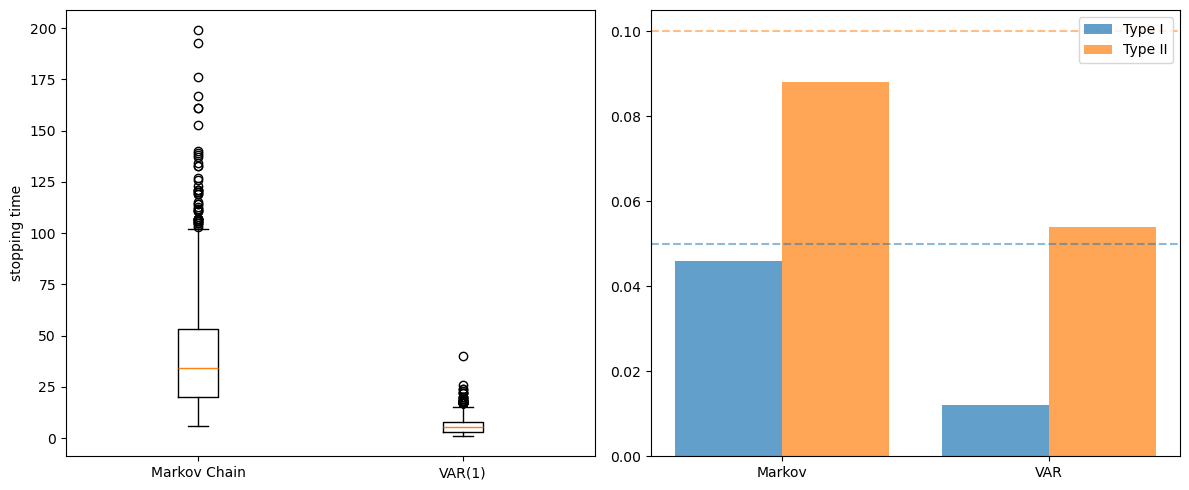
ax1.boxplot([results_markov['stopping_times'], 
             results_var['stopping_times']], 
           tick_labels=['Markov Chain', 'VAR(1)'])
ax1.set_ylabel('stopping time')

x = np.arange(2)
ax2.bar(x - 0.2, [results_markov['type_I'], results_var['type_I']], 
        0.4, label='Type I', alpha=0.7)
ax2.bar(x + 0.2, [results_markov['type_II'], results_var['type_II']], 
        0.4, label='Type II', alpha=0.7)
ax2.axhline(y=0.05, linestyle='--', alpha=0.5, color='C0')
ax2.axhline(y=0.10, linestyle='--', alpha=0.5, color='C1')
ax2.set_xticks(x), ax2.set_xticklabels(['Markov', 'VAR'])
ax2.legend() 
plt.tight_layout() 
plt.show()

_images/e2810c8bcf961b4e731d0a0d0076412de84cf3efd2dc8fc00a32b90d1c42b09d.png