81. Consumption Smoothing with Incomplete and Complete Markets#
81.1. Overview#
This lecture studies how the cross-section distribution of consumption evolves when many consumers each solve the LQ permanent income problem.
It is the second of three lectures on the LQ permanent income model and builds directly on The LQ Permanent Income Model.
We first show that the unit root in individual consumption causes the cross-section variance of consumption to grow linearly with time.
We then embed the individual consumer in a closed economy with a continuum of consumers, following Bewley [1977], and show how the gross interest rate \(R = \beta^{-1}\) emerges as an equilibrium outcome.
Finally, we replace the single risk-free bond with a complete set of Arrow securities and show how complete markets deliver a time-invariant cross-section distribution of consumption.
The third lecture, Robust Consumption Smoothing and Precautionary Savings, relaxes the assumption that the consumer fully trusts his income model.
Let’s begin with some imports.
import numpy as np
import matplotlib.pyplot as plt
from scipy.linalg import inv
81.2. A brief review#
We recall the essentials from The LQ Permanent Income Model.
A consumer with quadratic utility, discount factor \(\beta\), and access to a risk-free bond with gross return \(R = \beta^{-1}\) faces the endowment process
where \(w_{t+1}\) is IID with mean zero and identity covariance matrix.
The optimal consumption function expresses consumption as \(r/(1+r) = (1-\beta)\) times total wealth,
The model has a state-space representation in which the state is current consumption \(c_t\) and the exogenous endowment state \(z_t\):
Consumption is a random walk: its first difference is the IID innovation \(h\, w_{t+1}\), where \(h = (1-\beta)\,\check{G}(I-\beta\check{A})^{-1}\check{C}\).
Throughout we use the two-factor endowment \(y_t = z_{1t} + z_{2t}\) from The LQ Permanent Income Model, with \(z_{1t}\) a permanent component and \(z_{2t}\) a purely transitory component, so that \(\check{A} = \mathrm{diag}(1,0)\) and \(\check{C} = \mathrm{diag}(\sigma_1,\sigma_2)\).
The following cell reproduces the calibration and the key matrices.
# Parameters
β = 0.95       # discount factor (so R = 1/β)
σ1 = 0.15      # std of permanent shock
σ2 = 0.30      # std of transitory shock

# Two-factor endowment
A_check = np.array([[1.0, 0.0],
                    [0.0, 0.0]])
C_check = np.array([[σ1, 0.0],
                    [0.0, σ2]])
G_check = np.array([[1.0, 1.0]])

# Key matrix M = G(I - βA)^{-1}
IbA = np.eye(2) - β * A_check
M = G_check @ inv(IbA)   # shape (1, 2)
81.3. Spreading consumption cross sections#
The unit root in consumption (representation (81.3)) causes a cross-section variance of consumption to grow linearly with time.
Consider a continuum of ex ante identical households born at \(t = 0\).
All households \(i\) share the same preferences.
They all face a stochastic process for non-financial income of the same form
While all consumers face the same \(g\) process, they have different, statistically independent realizations of the idiosyncratic shock sequences \(\{w_{t}^i\}_{t=0}^\infty\).
Let all households start from the same initial conditions \(c_0^i = c_0\) and \(z_0^i\).
From (81.3), household \(i\)’s consumption follows
Since \(\{w^i_{t}\}\) realizations are independent across agents,
In the two-factor model, \(h\) is a \(1 \times 2\) row vector so \(hh^\top\) is a positive scalar equal to \(\sigma_1^2 + (1-\beta)^2\sigma_2^2\).
The cross-section variance of consumption grows like \(t\).
# Simulate cross-section spreading
rng = np.random.default_rng(42)
N = 5000       # number of agents
T_sim = 80         # number of periods

h_vec = (1 - β) * (M @ C_check)   # shape (1, 2), then flatten
h_vec = h_vec.flatten()            # h = [h1, h2]

c = np.zeros((N, T_sim + 1))       # consumption paths
# initialise all agents at c_0 = 0 (demeaned)
for t in range(T_sim):
    eps = rng.standard_normal((N, 2))    # N draws of 2D shock
    dc = eps @ h_vec              # shape (N,)
    c[:, t+1] = c[:, t] + dc

# Cross-section variance at each date
var_c = np.var(c, axis=0)
theory = np.arange(T_sim + 1) * np.dot(h_vec, h_vec)

fig, ax = plt.subplots()
ax.plot(var_c, label='simulated cross-section variance', lw=2)
ax.plot(theory, label=r'theoretical: $t \cdot h h^\top$',
        linestyle='--', color='C3', lw=2)
ax.set_xlabel('period $t$')
ax.set_ylabel('cross-section variance of $c$')
ax.legend()
plt.show()
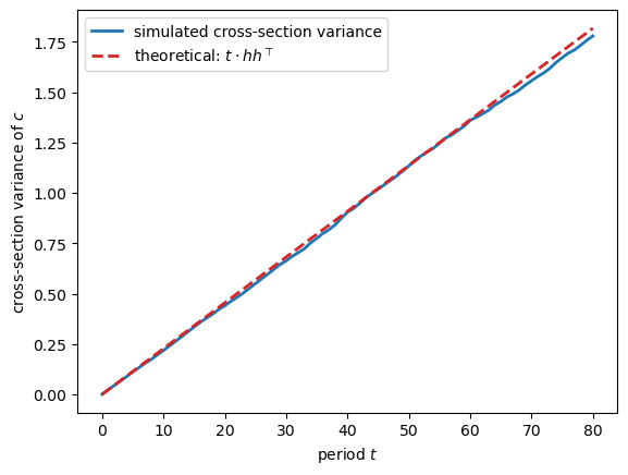
Fig. 81.1 Spreading consumption cross sections#
81.4. A borrowers and lenders economy#
Up to now we have set \(R = \beta^{-1}\) and taken it as determined outside the model (“small open economy”).
Following ideas of Bewley [1977], we can construct a closed economy in which \(R = \beta^{-1}\) is an equilibrium outcome.
A continuum of measure one of consumers, indexed by \(i \in [0,1]\), trade a risk-free one-period bond with price \(\beta\).
All consumers have the same preferences and the same stochastic income process (81.4), but face idiosyncratic non-financial income shock process realizations.
Initial bond positions are zero: \(b_0^i = 0\) for all \(i\).
Initial endowment states \(z_0^i\) are independent draws from a common initial distribution.
Because the permanent component \(z_{1t}\) has a unit root, process (81.1) has no stationary distribution, so in the simulation below we draw the permanent component \(z_{10}^i \sim N(0,1)\) and draw the transitory component \(z_{20}^i \sim N(0,\sigma_2^2)\) from its stationary distribution.
From (81.2), with \(b_0^i = 0\), agent \(i\)’s time-0 consumption is
For \(t \geq 1\), from (81.3):
Let \(Y\) denote the stationary mean of the cross-section average of non-financial income.
Integrating (81.6) over all agents:
because the continuum of idiosyncratic shocks averages to zero.
For future periods, integrating (81.7):
The goods market clears at every date at constant aggregate consumption equal to \(Y\).
The bond market clears at zero net supply each period.
Thus \(R = \beta^{-1}\) is an equilibrium outcome.
While the cross-section mean of consumption is constant, the cross-section variance grows without bound according to (81.5).
Initial differences in endowment draws \(z_0^i\) create permanent differences in consumption levels.
# Verify Bewley market clearing via simulation
# Online mean and variance avoid storing all paths.
rng = np.random.default_rng(0)
N_bew = 10000    # number of agents
T_bew = 60

# Draw initial states for the simulation.
z0_i = rng.standard_normal((N_bew, 2)) * np.array([1.0, σ2])
c0_i = ((1 - β) * (M @ z0_i.T)).flatten()   # shape (N_bew,)

# Propagate consumption across agents.
mean_c = np.zeros(T_bew + 1)
var_c2 = np.zeros(T_bew + 1)
mean_c[0] = c0_i.mean()
var_c2[0] = c0_i.var()

c_now = c0_i.copy()
for t in range(T_bew):
    eps = rng.standard_normal((N_bew, 2))
    c_now = c_now + eps @ h_vec
    mean_c[t + 1] = c_now.mean()
    var_c2[t + 1] = c_now.var()

# Reuse initial consumption below.
c_bew_t0 = c0_i

fig, axes = plt.subplots(1, 2, figsize=(12, 4))

axes[0].plot(mean_c, lw=2, color='C0')
axes[0].axhline(mean_c[0], linestyle='--', color='C3', label='initial mean')
axes[0].set_xlabel('period $t$')
axes[0].set_ylabel('mean consumption')
axes[0].set_title('mean')
axes[0].legend()

axes[1].plot(var_c2, lw=2, color='C0', label='simulated variance')
axes[1].set_xlabel('period $t$')
axes[1].set_ylabel('variance of consumption')
axes[1].set_title('variance')
axes[1].legend()
fig.tight_layout()
plt.show()
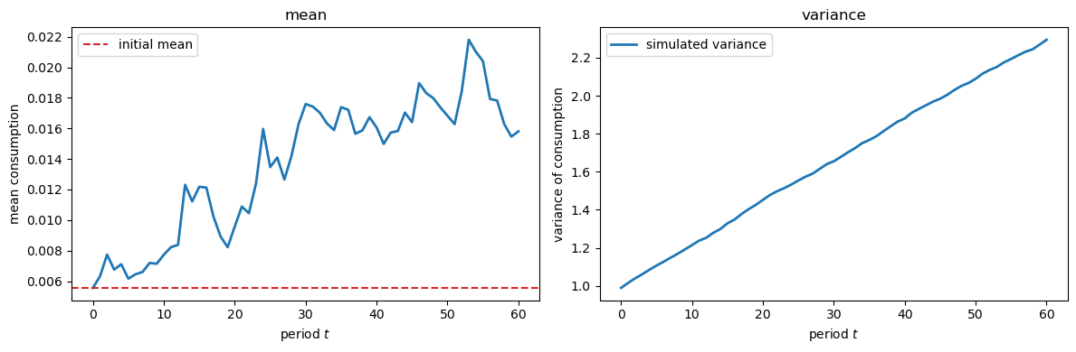
Fig. 81.2 Bewley economy cross-section moments#
Because each consumer dislikes variation of consumption over time, each consumer would prefer a completely smoothed stream \(c_t^i = c_0^i\) for all \(t\).
Such an allocation is feasible because the cross-section average of income is constant.
The next section describes a complete-markets allocation that supports this outcome.
81.5. Consumption smoothing with complete markets#
We replace the single bond with a complete set of Arrow securities.
The budget constraint becomes
where \(q(z_{t+1}|z_t)\) is the pricing kernel for one-period state-contingent claims and \(b_t(z_{t+1})\) is the household’s portfolio of Arrow securities chosen at \(t\).
We guess (and verify) that the equilibrium pricing kernel is
where \(\phi(z_{t+1}|z_t)\) is the transition density of \(z\).
This kernel prices a one-period risk-free bond at \(\beta\), so \(R = \beta^{-1}\), consistent with the incomplete-markets equilibrium.
We conjecture that the equilibrium delivers each consumer \(i\) a constant consumption level:
where \(c_0^i = (1-\beta)\,\check{G}(I-\beta\check{A})^{-1} z_0^i\) is the consumer’s time-0 consumption in the incomplete-markets economy.
The state-contingent debt that supports constant consumption is
Note that indebtedness depends only on the current Markov state \(z_t\), not on the history of earlier states.
This absence of history dependence reflects the complete risk sharing attained under complete markets.
Substituting the pricing kernel (81.10) and the portfolio conjecture (81.12) into the budget constraint (81.9) and using the law of iterated expectations confirms that the budget constraint simplifies to \(c_t = \bar{c}^i\) in every state and period.
Under complete markets, the cross-section distribution of consumption is time-invariant.
Consumer \(i\)’s rank in the consumption distribution is fixed forever.
A lucky initial draw \(z_0^i\) manifests itself as perpetually high consumption \(\bar{c}^i\) and lower indebtedness \(b(z_t^i, \bar{c}^i)\) across all future states.
This outcome contrasts with what happens in the incomplete-markets Bewley economy, where the cross-section variance of consumption grows without bound.
# Complete and incomplete consumption distributions
rng = np.random.default_rng(1)
N_cm = 5000
T_cm = 50

# Initial consumption draws (same as Bewley economy)
c0_cm = c_bew_t0[:N_cm]

# Incomplete markets: consumption evolves (random walk)
c_inc = np.zeros((N_cm, T_cm + 1))
c_inc[:, 0] = c0_cm
for t in range(T_cm):
    eps = rng.standard_normal((N_cm, 2))
    c_inc[:, t+1] = c_inc[:, t] + eps @ h_vec

# Complete markets: consumption stays constant
c_comp = np.tile(c0_cm[:, np.newaxis], T_cm + 1)

fig, axes = plt.subplots(1, 2, figsize=(12, 4))

for t_plot, color in zip([0, 10, 30, 50], ['C0', 'C1', 'C3', 'C4']):
    axes[0].hist(c_inc[:, t_plot], bins=60, alpha=0.4,
                 label=f't = {t_plot}', color=color, density=True)
axes[0].set_xlabel('$c$')
axes[0].set_ylabel('density, incomplete markets')
axes[0].set_title('incomplete markets')
axes[0].legend(fontsize=9)

for t_plot, color in zip([0, 10, 30, 50], ['C0', 'C1', 'C3', 'C4']):
    axes[1].hist(c_comp[:, t_plot], bins=60, alpha=0.4,
                 label=f't = {t_plot}', color=color, density=True)
axes[1].set_xlabel('$c$')
axes[1].set_ylabel('density, complete markets')
axes[1].set_title('complete markets')
axes[1].legend(fontsize=9)
fig.tight_layout()
plt.show()
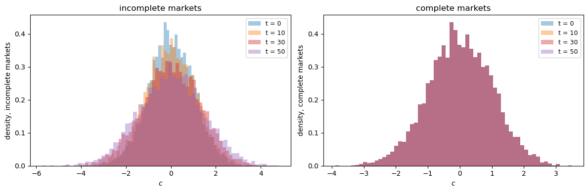
Fig. 81.3 Cross section distributions with incomplete and complete markets#
Note
Under complete markets the histogram stays the same across all \(t\) (distributions coincide perfectly), while under incomplete markets distributions spread out over time.
So far the consumer fully trusts his stochastic income model.
In Robust Consumption Smoothing and Precautionary Savings we relax that assumption and let the consumer seek decision rules that are robust to plausible misspecifications.
The optimal robust rule takes the same form as the rule above, but under a distorted model of the income process that looks more persistent than the approximating one.
81.6. Exercises#
Exercise 81.1
This exercise studies how patience governs the speed at which the cross-section of consumption spreads out.
From (81.5), the cross-section variance of consumption grows by \(h h^\top = \sigma_1^2 + (1-\beta)^2\sigma_2^2\) per period.
Compute this per-period growth rate for \(\beta \in \{0.90, 0.95, 0.99\}\) and report the permanent and transitory contributions separately.
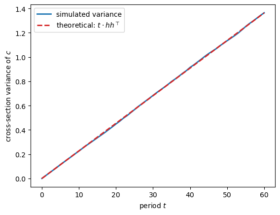
Confirm by simulation that the cross-section variance grows linearly at the predicted rate for \(\beta = 0.95\).
Explain why increasing \(\beta\) slows the spreading due to transitory shocks but leaves the contribution of permanent shocks unchanged.
Solution
Here is one solution:
for b in (0.90, 0.95, 0.99):
    perm = σ1**2
    tran = (1 - b)**2 * σ2**2
    print(f"β = {b}:  growth = {perm + tran:.5f}  "
          f"(permanent {perm:.5f}, transitory {tran:.5f})")
β = 0.9:  growth = 0.02340  (permanent 0.02250, transitory 0.00090)
β = 0.95:  growth = 0.02272  (permanent 0.02250, transitory 0.00023)
β = 0.99:  growth = 0.02251  (permanent 0.02250, transitory 0.00001)
rng = np.random.default_rng(7)
N, T_sim = 20000, 60
hh = float(h_vec @ h_vec)

c = np.zeros((N, T_sim + 1))
for t in range(T_sim):
    c[:, t + 1] = c[:, t] + rng.standard_normal((N, 2)) @ h_vec

var_c = c.var(axis=0)
theory = np.arange(T_sim + 1) * hh

fig, ax = plt.subplots()
ax.plot(var_c, lw=2, label='simulated variance')
ax.plot(theory, lw=2, linestyle='--', color='C3',
        label=r'theoretical: $t\cdot h h^\top$')
ax.set_xlabel('period $t$')
ax.set_ylabel('cross-section variance of $c$')
ax.legend()
plt.show()
The permanent contribution \(\sigma_1^2\) does not depend on \(\beta\) because a permanent shock is capitalised one-for-one into consumption regardless of patience.
The transitory contribution \((1-\beta)^2\sigma_2^2\) shrinks as \(\beta \to 1\) because a more patient consumer smooths a transitory shock over a longer horizon, moving consumption by only the small annuity value \((1-\beta)\).
Exercise 81.2
This exercise contrasts the cross-section variance of consumption under incomplete and complete markets.
Start all consumers from the initial consumption draws c_bew_t0 computed above.
Compute the cross-section variance at each date \(t = 0, 1, \ldots, 60\) under incomplete markets (consumption is a random walk) and under complete markets (consumption is constant).
Plot the two variance paths on the same axes and comment on the difference.
Solution
Here is one solution:
rng = np.random.default_rng(11)
T = 60
c0 = c_bew_t0

# Incomplete markets: random-walk consumption
c_inc = np.zeros((len(c0), T + 1))
c_inc[:, 0] = c0
for t in range(T):
    c_inc[:, t + 1] = c_inc[:, t] + rng.standard_normal((len(c0), 2)) @ h_vec

var_inc = c_inc.var(axis=0)
var_comp = np.full(T + 1, c0.var())   # complete markets: constant consumption

fig, ax = plt.subplots()
ax.plot(var_inc, lw=2, label='incomplete markets')
ax.plot(var_comp, lw=2, linestyle='--', color='C3', label='complete markets')
ax.set_xlabel('period $t$')
ax.set_ylabel('cross-section variance of $c$')
ax.legend()
plt.show()
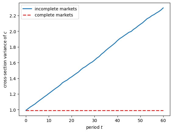
Under incomplete markets the variance rises linearly without bound: each consumer accumulates an independent random walk of consumption innovations.
Under complete markets the variance is flat: each consumer locks in a constant consumption level \(\bar{c}^i\), so the cross-section distribution never changes.
Exercise 81.3
This exercise shows how complete markets freeze each consumer’s rank in the consumption distribution.
Under complete markets consumption is constant, so a consumer’s position in the cross-section distribution never changes; under incomplete markets the random walk gradually scrambles ranks.
Simulate consumption paths under both market structures, starting from
c_bew_t0.Compute the Spearman rank correlation between consumption at \(t = 0\) and at later dates \(t\) under each market structure, and plot it against \(t\).
Interpret the result.
Solution
Here is one solution:
from scipy.stats import spearmanr

rng = np.random.default_rng(3)
T = 60
c0 = c_bew_t0

c_inc = np.zeros((len(c0), T + 1))
c_inc[:, 0] = c0
for t in range(T):
    c_inc[:, t + 1] = c_inc[:, t] + rng.standard_normal((len(c0), 2)) @ h_vec

dates = np.arange(0, T + 1, 4)
rank_inc = [spearmanr(c_inc[:, 0], c_inc[:, t]).statistic for t in dates]
rank_comp = [1.0 for _ in dates]   # constant consumption ⇒ ranks fixed

fig, ax = plt.subplots()
ax.plot(dates, rank_comp, lw=2, linestyle='--', color='C3',
        label='complete markets')
ax.plot(dates, rank_inc, lw=2, marker='o', color='C0',
        label='incomplete markets')
ax.set_xlabel('period $t$')
ax.set_ylabel(r'rank correlation with $c_0$')
ax.set_ylim(0, 1.05)
ax.legend()
plt.show()
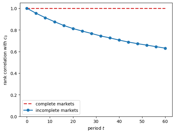
Under complete markets the rank correlation stays exactly one: each consumer keeps the rank determined by the initial draw \(z_0^i\) forever.
Under incomplete markets the rank correlation decays toward zero as the accumulated random walk reshuffles who is rich and who is poor, even though every consumer faces the same income process.