65. Stability in Linear Rational Expectations Models#

65.1. Overview#

This lecture studies stability in the context of an elementary rational expectations model.

We study a rational expectations version of Philip Cagan’s model [Cagan, 1956] linking the price level to the money supply.

Cagan did not use a rational expectations version of his model, but Sargent [Sargent, 1977] did.

We study a rational expectations version of this model because it is intrinsically interesting and because it has a mathematical structure that appears in virtually all linear rational expectations model, namely, that a key endogenous variable equals a mathematical expectation of a geometric sum of future values of another variable.

The model determines the price level or rate of inflation as a function of the money supply or the rate of change in the money supply.

In this lecture, we’ll encounter:

• a convenient formula for the expectation of geometric sum of future values of a variable

• a way of solving an expectational difference equation by mapping it into a vector first-order difference equation and appropriately manipulating an eigen decomposition of the transition matrix in order to impose stability

• a way to use a Big $K$, little $k$ argument to allow apparent feedback from endogenous to exogenous variables within a rational expectations equilibrium

• a use of eigenvector decompositions of matrices that allowed Blanchard and Khan (1981) [Blanchard and Kahn, 1980] and Whiteman (1983) [Whiteman, 1983] to solve a class of linear rational expectations models

• how to use SymPy to get analytical formulas for some key objects comprising a rational expectations equilibrium

Matrix decompositions employed here are described in more depth in this lecture Lagrangian formulations.

We formulate a version of Cagan’s model under rational expectations as an expectational difference equation whose solution is a rational expectations equilibrium.

We’ll start this lecture with a quick review of deterministic (i.e., non-random) first-order and second-order linear difference equations.

65.2. Linear Difference Equations#

We’ll use the backward shift or lag operator $L$.

The lag operator $L$ maps a sequence $\{x_t{\}}_{t=0}^{\mathrm{\infty }}$ into the sequence $\{x_{t-1}{\}}_{t=0}^{\mathrm{\infty }}$

We’ll deploy $L$ by using the equality $L{x}_t\equiv x_{t-1}$ in algebraic expressions.

Further, the inverse $L^{-1}$ of the lag operator is the forward shift operator.

We’ll often use the equality $L^{-1}{x}_t\equiv x_{t+1}$ below.

The algebra of lag and forward shift operators can simplify representing and solving linear difference equations.

65.3. Illustration: Cagan’s Model#

Now let’s use linear difference equations to represent and solve Sargent’s [Sargent, 1977] rational expectations version of Cagan’s model [Cagan, 1956] that connects the price level to the public’s anticipations of future money supplies.

Cagan did not use a rational expectations version of his model, but Sargent [Sargent, 1977]

Let

• $m_t^d$ be the log of the demand for money

• $m_t$ be the log of the supply of money

• $p_t$ be the log of the price level

It follows that $p_{t+1}-p_t$ is the rate of inflation.

The logarithm of the demand for real money balances $m_t^d-p_t$ is an inverse function of the expected rate of inflation $p_{t+1}-p_t$ for $t\ge 0$:

Equate the demand for log money $m_t^d$ to the supply of log money $m_t$ in the above equation and rearrange to deduce that the logarithm of the price level $p_t$ is related to the logarithm of the money supply $m_t$ by

where $\lambda \equiv \frac{\beta }{1+\beta }\in (0,1)$.

(We note that the characteristic polynomial if $1-{\lambda }^{-1}{z}^{-1}=0$ so that the zero of the characteristic polynomial in this case is $\lambda \in (0,1)$ which here is inside the unit circle.)

Solving the first order difference equation (65.8) forward gives

which is the unique stable solution of difference equation (65.8) among a class of more general solutions

that is indexed by the real number $c\in \mathbf{R}$.

Because we want to focus on stable solutions, we set $c=0$.

Equation (65.10) attributes perfect foresight about the money supply sequence to the holders of real balances.

We begin by assuming that the log of the money supply is exogenous in the sense that it is an autonomous process that does not feed back on the log of the price level.

In particular, we assume that the log of the money supply is described by the linear state space system

where $x_t$ is an $n\times 1$ vector that does not include $p_t$ or lags of $p_t$, $A$ is an $n\times n$ matrix with eigenvalues that are less than ${\lambda }^{-1}$ in absolute values, and $G$ is a $1\times n$ selector matrix.

Variables appearing in the vector $x_t$ contain information that might help predict future values of the money supply.

We’ll start with an example in which $x_t$ includes only $m_t$, possibly lagged values of $m$, and a constant.

An example of such an $\{m_t\}$ process that fits info state space system (65.11) is one that satisfies the second order linear difference equation

where the zeros of the characteristic polynomial $(1-{\rho }_{1}z-{\rho }_2{z}^2)$ are strictly greater than $1$ in modulus.

(Please see this QuantEcon lecture for more about characteristic polynomials and their role in solving linear difference equations.)

We seek a stable or non-explosive solution of the difference equation (65.8) that obeys the system comprised of (65.8)-(65.11).

By stable or non-explosive, we mean that neither $m_t$ nor $p_t$ diverges as $t\to +\mathrm{\infty }$.

This requires that we shut down the term $c{\lambda }^{-t}$ in equation (65.10) above by setting $c=0$

The solution we are after is

where

65.4. Some Python Code#

We’ll construct examples that illustrate (65.11).

Our first example takes as the law of motion for the log money supply the second order difference equation

that is parameterized by ${\rho }_1,{\rho }_2,\alpha$

To capture this parameterization with system (65.9) we set

Here is Python code

λ = .9

α = 0
ρ1 = .9
ρ2 = .05

A = np.array([[1,  0,  0],
              [α, ρ1, ρ2],
              [0,  1,  0]])
G = np.array([[0, 1, 0]])

The matrix $A$ has one eigenvalue equal to unity.

It is associated with the $A_{11}$ component that captures a constant component of the state $x_t$.

We can verify that the two eigenvalues of $A$ not associated with the constant in the state $x_t$ are strictly less than unity in modulus.

eigvals = np.linalg.eigvals(A)
print(eigvals)

[-0.05249378  0.95249378  1.        ]

(abs(eigvals) <= 1).all()

True

Now let’s compute $F$ in formulas (65.12) and (65.13).

# compute the solution, i.e. forumula (3)
F = (1 - λ) * G @ np.linalg.inv(np.eye(A.shape[0]) - λ * A)
print("F= ",F)

F=  [[0.         0.66889632 0.03010033]]

Now let’s simulate paths of $m_t$ and $p_t$ starting from an initial value $x_0$.

# set the initial state
x0 = np.array([1, 1, 0])

T = 100 # length of simulation

m_seq = np.empty(T+1)
p_seq = np.empty(T+1)

[m_seq[0]] = G @ x0
[p_seq[0]] = F @ x0

# simulate for T periods
x_old = x0
for t in range(T):

    x = A @ x_old

    [m_seq[t+1]] = G @ x
    [p_seq[t+1]] = F @ x

    x_old = x

plt.figure()
plt.plot(range(T+1), m_seq, label=r'$m_t$')
plt.plot(range(T+1), p_seq, label=r'$p_t$')
plt.xlabel('t')
plt.title(rf'λ={λ}, α={α}, $ρ_1$={ρ1}, $ρ_2$={ρ2}')
plt.legend()
plt.show()

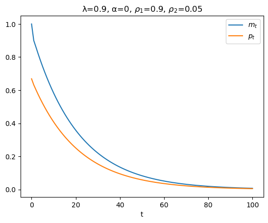
In the above graph, why is the log of the price level always less than the log of the money supply?

Because

• according to equation (65.9), $p_t$ is a geometric weighted average of current and future values of $m_t$, and

• it happens that in this example future $m$’s are always less than the current $m$

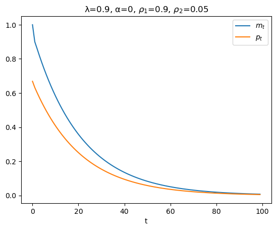
65.5. Alternative Code#

We could also have run the simulation using the quantecon LinearStateSpace code.

The following code block performs the calculation with that code.

# construct a LinearStateSpace instance

# stack G and F
G_ext = np.vstack([G, F])

C = np.zeros((A.shape[0], 1))

ss = qe.LinearStateSpace(A, C, G_ext, mu_0=x0)

T = 100

# simulate using LinearStateSpace
x, y = ss.simulate(ts_length=T)

# plot
plt.figure()
plt.plot(range(T), y[0,:], label='$m_t$')
plt.plot(range(T), y[1,:], label='$p_t$')
plt.xlabel('t')
plt.title(f'λ={λ}, α={α}, $ρ_1$={ρ1}, $ρ_2$={ρ2}')
plt.legend()
plt.show()

65.6. Another Perspective#

Above, we imposed stability or non-explosiveness on the solution of the key difference equation (65.8) in Cagan’s model by solving the unstable root of the characteristic polynomial forward.

To shed light on the mechanics involved in imposing stability on a solution of a potentially unstable system of linear difference equations and to prepare the way for generalizations of our model in which the money supply is allowed to feed back on the price level itself, we stack equations (65.8) and (65.15) to form the system

or

where

Transition matrix $H$ has eigenvalues $\rho \in (0,1)$ and ${\lambda }^{-1}>1$.

Because an eigenvalue of $H$ exceeds unity, if we iterate on equation (65.17) starting from an arbitrary initial vector $y_0=\left[\begin{array}{c}{m}_0\\ p_0\end{array}\right]$ with $m_0>0,p_0>0$, we discover that in general absolute values of both components of $y_t$ diverge toward $+\mathrm{\infty }$ as $t\to +\mathrm{\infty }$.

To substantiate this claim, we can use the eigenvector matrix decomposition of $H$ that is available to us because the eigenvalues of $H$ are distinct

Here $\mathrm{\Lambda }$ is a diagonal matrix of eigenvalues of $H$ and $Q$ is a matrix whose columns are eigenvectors associated with the corresponding eigenvalues.

Note that

so that

For almost all initial vectors $y_0$, the presence of the eigenvalue ${\lambda }^{-1}>1$ causes both components of $y_t$ to diverge in absolute value to $+\mathrm{\infty }$.

To explore this outcome in more detail, we can use the following transformation

that allows us to represent the dynamics in a way that isolates the source of the propensity of paths to diverge:

Staring at this equation indicates that unless

the path of $y_t^{\ast }$ and therefore the paths of both components of $y_t=Q{y}_t^{\ast }$ will diverge in absolute value as $t\to +\mathrm{\infty }$. (We say that the paths explode)

Equation (65.19) also leads us to conclude that there is a unique setting for the initial vector $y_0$ for which both components of $y_t$ do not diverge.

The required setting of $y_0$ must evidently have the property that

But note that since $y_0=\left[\begin{array}{c}{m}_0\\ p_0\end{array}\right]$ and $m_0$ is given to us an initial condition, $p_0$ has to do all the adjusting to satisfy this equation.

Sometimes this situation is described by saying that while $m_0$ is truly a state variable, $p_0$ is a jump variable that must adjust at $t=0$ in order to satisfy the equation.

Thus, in a nutshell the unique value of the vector $y_0$ for which the paths of $y_t$ do not diverge must have second component $p_0$ that verifies equality (65.19) by setting the second component of $y_0^{\ast }$ equal to zero.

The component $p_0$ of the initial vector $y_0=\left[\begin{array}{c}{m}_0\\ p_0\end{array}\right]$ must evidently satisfy

where $Q^{\{2\}}$ denotes the second row of $Q^{-1}$, a restriction that is equivalent to

where $Q^{ij}$ denotes the $(i,j)$ component of $Q^{-1}$.

Solving this equation for $p_0$, we find

This is the unique stabilizing value of $p_0$ expressed as a function of $m_0$.

65.7. Log money Supply Feeds Back on Log Price Level#

An arrangement of eigenvalues that split around unity, with one being below unity and another being greater than unity, sometimes prevails when there is feedback from the log price level to the log money supply.

Let the feedback rule be

where $\rho \in (0,1)$ and where we shall now allow $\delta \ne 0$.

Warning: If things are to fit together as we wish to deliver a stable system for some initial value $p_0$ that we want to determine uniquely, $\delta$ cannot be too large.

The forward-looking equation (65.8) continues to describe equality between the demand and supply of money.

We assume that equations (65.8) and (65.24) govern $y_t\equiv \left[\begin{array}{c}{m}_t\\ p_t\end{array}\right]$ for $t\ge 0$.

The transition matrix $H$ in the law of motion

now becomes

We take $m_0$ as a given initial condition and as before seek an initial value $p_0$ that stabilizes the system in the sense that $y_t$ converges as $t\to +\mathrm{\infty }$.

Our approach is identical with the one followed above and is based on an eigenvalue decomposition in which, cross our fingers, one eigenvalue exceeds unity and the other is less than unity in absolute value.

When $\delta \ne 0$ as we now assume, the eigenvalues of $H$ will no longer be $\rho \in (0,1)$ and ${\lambda }^{-1}>1$

We’ll just calculate them and apply the same algorithm that we used above.

That algorithm remains valid so long as the eigenvalues split around unity as before.

Again we assume that $m_0$ is an initial condition, but that $p_0$ is not given but to be solved for.

Let’s write and execute some Python code that will let us explore how outcomes depend on $\delta$.

def construct_H(ρ, λ, δ):
    "contruct matrix H given parameters."

    H = np.empty((2, 2))
    H[0, :] = ρ,δ
    H[1, :] = - (1 - λ) / λ, 1 / λ

    return H

def H_eigvals(ρ=.9, λ=.5, δ=0):
    "compute the eigenvalues of matrix H given parameters."

    # construct H matrix
    H = construct_H(ρ, λ, δ)

    # compute eigenvalues
    eigvals = np.linalg.eigvals(H)

    return eigvals

H_eigvals()

array([2. , 0.9])

Notice that a negative $\delta$ will not imperil the stability of the matrix $H$, even if it has a big absolute value.

# small negative δ
H_eigvals(δ=-0.05)

array([0.8562829, 2.0437171])

# large negative δ
H_eigvals(δ=-1.5)

array([0.10742784, 2.79257216])

A sufficiently small positive $\delta$ also causes no problem.

# sufficiently small positive δ
H_eigvals(δ=0.05)

array([0.94750622, 1.95249378])

But a large enough positive $\delta$ makes both eigenvalues of $H$ strictly greater than unity in modulus.

For example,

H_eigvals(δ=0.2)

array([1.12984379, 1.77015621])

We want to study systems in which one eigenvalue exceeds unity in modulus while the other is less than unity in modulus, so we avoid values of $\delta$ that are too.

That is, we want to avoid too much positive feedback from $p_t$ to $m_{t+1}$.

def magic_p0(m0, ρ=.9, λ=.5, δ=0):
    """
    Use the magic formula (8) to compute the level of p0
    that makes the system stable.
    """

    H = construct_H(ρ, λ, δ)
    eigvals, Q = np.linalg.eig(H)

    # find the index of the smaller eigenvalue
    ind = 0 if eigvals[0] < eigvals[1] else 1

    # verify that the eigenvalue is less than unity
    if eigvals[ind] > 1:

        print("both eigenvalues exceed unity in modulus")

        return None

    p0 = Q[1, ind] / Q[0, ind] * m0

    return p0

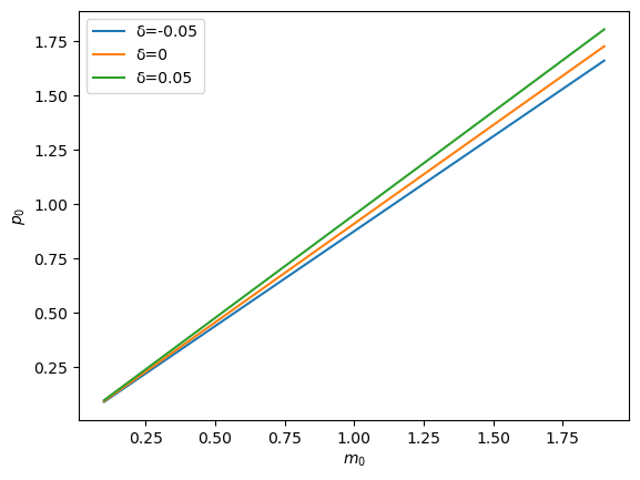
Let’s plot how the solution $p_0$ changes as $m_0$ changes for different settings of $\delta$.

m_range = np.arange(0.1, 2., 0.1)

for δ in [-0.05, 0, 0.05]:
    plt.plot(m_range, [magic_p0(m0, δ=δ) for m0 in m_range], label=f"δ={δ}")
plt.legend()

plt.xlabel(r"$m_0$")
plt.ylabel(r"$p_0$")
plt.show()

To look at things from a different angle, we can fix the initial value $m_0$ and see how $p_0$ changes as $\delta$ changes.

m0 = 1

δ_range = np.linspace(-0.05, 0.05, 100)
plt.plot(δ_range, [magic_p0(m0, δ=δ) for δ in δ_range])
plt.xlabel(r'$\delta$')
plt.ylabel(r'$p_0$')
plt.title(rf'$m_0$={m0}')
plt.show()

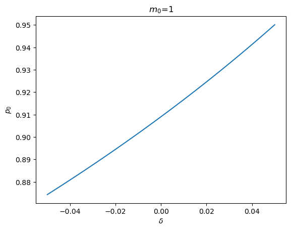
Notice that when $\delta$ is large enough, both eigenvalues exceed unity in modulus, causing a stabilizing value of $p_0$ not to exist.

magic_p0(1, δ=0.2)

both eigenvalues exceed unity in modulus

65.8. Big $P$, Little $p$ Interpretation#

It is helpful to view our solutions of difference equations having feedback from the price level or inflation to money or the rate of money creation in terms of the Big $K$, little $k$ idea discussed in Rational Expectations Models.

This will help us sort out what is taken as given by the decision makers who use the difference equation (65.9) to determine $p_t$ as a function of their forecasts of future values of $m_t$.

Let’s write the stabilizing solution that we have computed using the eigenvector decomposition of $H$ as $P_t=F^{\ast }{m}_t$, where

Then from $P_{t+1}=F^{\ast }{m}_{t+1}$ and $m_{t+1}=\rho m_t+\delta P_t$ we can deduce the recursion $P_{t+1}=F^{\ast }\rho m_t+F^{\ast }\delta P_t$ and create the stacked system

or

where $x_t=\left[\begin{array}{c}{m}_t\\ P_t\end{array}\right]$.

Apply formula (65.13) for $F$ to deduce that

which implies that

so that we can anticipate that

We shall verify this equality in the next block of Python code that implements the following computations.

1. For the system with $\delta \ne 0$ so that there is feedback, we compute the stabilizing solution for $p_t$ in the form $p_t=F^{\ast }{m}_t$ where $F^{\ast }=Q_{21}{Q}_{11}^{-1}$ as above.

2. Recalling the system (65.11), (65.12), and (65.13) above, we define $x_t=\left[\begin{array}{c}{m}_t\\ P_t\end{array}\right]$ and notice that it is Big $P_t$ and not little $p_t$ here. Then we form $A$ and $G$ as $A=\left[\begin{array}{cc}\rho & \delta \\ F^{\ast }\rho & F^{\ast }\delta \end{array}\right]$ and $G=\left[\begin{array}{cc}1& 0\end{array}\right]$ and we compute $\left[\begin{array}{cc}{F}_1& F_2\end{array}\right]\equiv F$ from equation (65.13) above.

3. We compute $F_1+F_2{F}^{\ast }$ and compare it with $F^{\ast }$ and check for the anticipated equality.

# set parameters
ρ = .9
λ = .5
δ = .05

# solve for F_star
H = construct_H(ρ, λ, δ)
eigvals, Q = np.linalg.eig(H)

ind = 0 if eigvals[0] < eigvals[1] else 1
F_star = Q[1, ind] / Q[0, ind]
F_star

# solve for F_check
A = np.empty((2, 2))
A[0, :] = ρ, δ
A[1, :] = F_star * A[0, :]

G = np.array([1, 0])

F_check= (1 - λ) * G @ np.linalg.inv(np.eye(2) - λ * A)
F_check

array([0.92755597, 0.02375311])

Compare $F^{\ast }$ with $F_1+F_2{F}^{\ast }$

F_check[0] + F_check[1] * F_star, F_star

65.9. Fun with SymPy#

This section is a gift for readers who have made it this far.

It puts SymPy to work on our model.

Thus, we use Sympy to compute some key objects comprising the eigenvector decomposition of $H$.

We start by generating an $H$ with nonzero $\delta$.

λ, δ, ρ = symbols('λ, δ, ρ')

H1 = Matrix([[ρ,δ], [- (1 - λ) / λ, λ ** -1]])

H1

H1.eigenvals()

H1.eigenvects()

Now let’s compute $H$ when $\delta$ is zero.

H2 = Matrix([[ρ,0], [- (1 - λ) / λ, λ ** -1]])

H2

H2.eigenvals()

H2.eigenvects()

Below we do induce SymPy to do the following fun things for us analytically:

1. We compute the matrix $Q$ whose first column is the eigenvector associated with $\rho$. and whose second column is the eigenvector associated with ${\lambda }^{-1}$.

2. We use SymPy to compute the inverse $Q^{-1}$ of $Q$ (both in symbols).

3. We use SymPy to compute $Q_{21}{Q}_{11}^{-1}$ (in symbols).

4. Where $Q^{ij}$ denotes the $(i,j)$ component of $Q^{-1}$, we use SymPy to compute $-(Q^{22}{)}^{-1}{Q}^{21}$ (again in symbols)

# construct Q
vec = []
for i, (eigval, _, eigvec) in enumerate(H2.eigenvects()):

    vec.append(eigvec[0])

    if eigval == ρ:
        ind = i

Q = vec[ind].col_insert(1, vec[1-ind])

Q

$Q^{-1}$

Q_inv = Q ** (-1)
Q_inv

$Q_{21}{Q}_{11}^{-1}$

Q[1, 0] / Q[0, 0]

$-(Q^{22}{)}^{-1}{Q}^{21}$

- Q_inv[1, 0] / Q_inv[1, 1]