84. Cass-Koopmans Model#
84.1. Overview#
This lecture and Cass-Koopmans Competitive Equilibrium describe a model that Tjalling Koopmans [Koopmans, 1965] and David Cass [Cass, 1965] used to analyze optimal growth.
The model extends the model of Robert Solow described in an earlier lecture.
It does so by making saving rate be a decision, instead of a hard-wired constant.
(Solow assumed a constant saving rate determined outside the model.)
We describe two versions of the model, a planning problem in this lecture, and a competitive equilibrium in this lecture Cass-Koopmans Competitive Equilibrium.
Together, the two lectures illustrate what is, in fact, a more general connection between a planned economy and a decentralized economy organized as a competitive equilibrium.
This lecture is devoted to the planned economy version.
In the planned economy, there are
no prices
no budget constraints
Instead there is a dictator that tells people
what to produce
what to invest in physical capital
who is to consume what and when
The lecture uses important ideas including
A min-max problem for solving a planning problem.
A shooting algorithm for solving difference equations subject to initial and terminal conditions.
A turnpike property of optimal paths for long but finite-horizon economies.
A stable manifold and a phase plane
In addition to what’s in Anaconda, this lecture will need the following libraries:
!pip install quantecon
Let’s start with some standard imports:
import matplotlib.pyplot as plt
from numba import jit, float64
from numba.experimental import jitclass
import numpy as np
from quantecon.optimize import brentq
84.2. The Model#
Time is discrete and takes values \(t = 0, 1 , \ldots, T\) where \(T\) is finite.
(We’ll eventually study a limiting case in which \(T = + \infty\))
A single good can either be consumed or invested in physical capital.
The consumption good is not durable and depreciates completely if not consumed immediately.
The capital good is durable but depreciates.
We let \(C_t\) be the total consumption of a nondurable consumption good at time \(t\).
Let \(K_t\) be the stock of physical capital at time \(t\).
Let \(\vec{C}\) = \(\{C_0,\dots, C_T\}\) and \(\vec{K}\) = \(\{K_0,\dots,K_{T+1}\}\).
84.2.1. Digression: Aggregation Theory#
We use a concept of a representative consumer to be thought of as follows.
There is a unit mass of identical consumers indexed by \(\omega \in [0,1]\).
Consumption of consumer \(\omega\) is \(c(\omega)\).
Aggregate consumption is
Consider a welfare problem that chooses an allocation \(\{c(\omega)\}\) across consumers to maximize
where \(u(\cdot)\) is a concave utility function with \(u' >0, u'' < 0\) and maximization is subject to
Form a Lagrangian \(L = \int_0^1 u(c(\omega)) d \omega + \lambda [C - \int_0^1 c(\omega) d \omega ] \).
Differentiate under the integral signs with respect to each \(\omega\) to obtain the first-order necessary conditions
These conditions imply that \(c(\omega)\) equals a constant \(c\) that is independent of \(\omega\).
To find \(c\), use feasibility constraint (84.1) to conclude that
This line of argument indicates the special aggregation theory that lies beneath outcomes in which a representative consumer consumes amount \(C\).
It appears often in aggregate economics.
We shall use this aggregation theory here and also in this lecture Cass-Koopmans Competitive Equilibrium.
84.2.1.1. An Economy#
A representative household is endowed with one unit of labor at each \(t\) and likes the consumption good at each \(t\).
The representative household inelastically supplies a single unit of labor \(N_t\) at each \(t\), so that \(N_t =1 \text{ for all } t \in \{0, 1, \ldots, T\}\).
The representative household has preferences over consumption bundles ordered by the utility functional:
where \(\beta \in (0,1)\) is a discount factor and \(\gamma >0\) governs the curvature of the one-period utility function.
Larger \(\gamma\)’s imply more curvature.
Note that
satisfies \(u'>0,u''<0\).
\(u' > 0\) asserts that the consumer prefers more to less.
\(u''< 0\) asserts that marginal utility declines with increases in \(C_t\).
We assume that \(K_0 > 0\) is an exogenous initial capital stock.
There is an economy-wide production function
with \(0 < \alpha<1\), \(A > 0\).
A feasible allocation \(\vec{C}, \vec{K}\) satisfies
where \(\delta \in (0,1)\) is a depreciation rate of capital.
84.3. Planning Problem#
A planner chooses an allocation \(\{\vec{C},\vec{K}\}\) to maximize (84.2) subject to (84.5).
Let \(\vec{\mu}=\{\mu_0,\dots,\mu_T\}\) be a sequence of nonnegative Lagrange multipliers.
To find an optimal allocation, form a Lagrangian
and pose the following min-max problem:
Extremization means maximization with respect to \(\vec{C}, \vec{K}\) and minimization with respect to \(\vec{\mu}\).
Our problem satisfies conditions that assure that second-order conditions are satisfied at an allocation that satisfies the first-order necessary conditions that we are about to compute.
Before computing first-order conditions, we present some handy formulas.
84.3.1. Useful Properties of Linearly Homogeneous Production Function#
The following technicalities will help us.
Notice that
Define the output per-capita production function
whose argument is capital per-capita.
It is useful to recall the following calculations for the marginal product of capital
and the marginal product of labor
(Here we are using that \(N_t = 1\) for all \(t\), so that \(K_t = \frac{K_t}{N_t}\).)
84.3.2. First-order necessary conditions#
We now compute first-order necessary conditions for extremization of Lagrangian (84.6):
In computing (84.10) we recognize that \(K_t\) appears in both the time \(t\) and time \(t-1\) feasibility constraints (84.5).
Restrictions (84.12) come from differentiating with respect to \(K_{T+1}\) and applying the following Karush-Kuhn-Tucker condition (KKT) (see Karush-Kuhn-Tucker conditions):
Combining (84.9) and (84.10) gives
which can be rearranged to become
Applying the inverse marginal utility of consumption function on both sides of the above equation gives
which for our utility function (84.3) becomes the consumption Euler equation
which we can combine with the feasibility constraint (84.5) to get
This is a pair of non-linear first-order difference equations that map \(C_t, K_t\) into \(C_{t+1}, K_{t+1}\) and that an optimal sequence \(\vec C , \vec K\) must satisfy.
It must also satisfy the initial condition that \(K_0\) is given and \(K_{T+1} = 0\).
Below we define a jitclass that stores parameters and functions
that define our economy.
planning_data = [
    ('γ', float64),    # Coefficient of relative risk aversion
    ('β', float64),    # Discount factor
    ('δ', float64),    # Depreciation rate on capital
    ('α', float64),    # Return to capital per capita
    ('A', float64)     # Technology
]
@jitclass(planning_data)
class PlanningProblem():

    def __init__(self, γ=2, β=0.95, δ=0.02, α=0.33, A=1):

        self.γ, self.β = γ, β
        self.δ, self.α, self.A = δ, α, A

    def u(self, c):
        '''
        Utility function
        ASIDE: If you have a utility function that is hard to solve by hand
        you can use automatic or symbolic differentiation
        See https://github.com/HIPS/autograd
        '''
        γ = self.γ

        return c ** (1 - γ) / (1 - γ) if γ!= 1 else np.log(c)

    def u_prime(self, c):
        'Derivative of utility'
        γ = self.γ

        return c ** (-γ)

    def u_prime_inv(self, c):
        'Inverse of derivative of utility'
        γ = self.γ

        return c ** (-1 / γ)

    def f(self, k):
        'Production function'
        α, A = self.α, self.A

        return A * k ** α

    def f_prime(self, k):
        'Derivative of production function'
        α, A = self.α, self.A

        return α * A * k ** (α - 1)

    def f_prime_inv(self, k):
        'Inverse of derivative of production function'
        α, A = self.α, self.A

        return (k / (A * α)) ** (1 / (α - 1))

    def next_k_c(self, k, c):
        ''''
        Given the current capital Kt and an arbitrary feasible
        consumption choice Ct, computes Kt+1 by state transition law
        and optimal Ct+1 by Euler equation.
        '''
        β, δ = self.β, self.δ
        u_prime, u_prime_inv = self.u_prime, self.u_prime_inv
        f, f_prime = self.f, self.f_prime

        k_next = f(k) + (1 - δ) * k - c
        c_next = u_prime_inv(u_prime(c) / (β * (f_prime(k_next) + (1 - δ))))

        return k_next, c_next
We can construct an economy with the Python code:
pp = PlanningProblem()
84.4. Shooting Algorithm#
We use shooting to compute an optimal allocation \(\vec{C}, \vec{K}\) and an associated Lagrange multiplier sequence \(\vec{\mu}\).
First-order necessary conditions (84.9), (84.10), and (84.11) for the planning problem form a system of difference equations with two boundary conditions:
\(K_0\) is a given initial condition for capital
\(K_{T+1} =0\) is a terminal condition for capital that we deduced from the first-order necessary condition for \(K_{T+1}\) the KKT condition (84.13)
We have no initial condition for the Lagrange multiplier \(\mu_0\).
If we did, our job would be easy:
Given \(\mu_0\) and \(k_0\), we could compute \(c_0\) from equation (84.9) and then \(k_1\) from equation (84.11) and \(\mu_1\) from equation (84.10).
We could continue in this way to compute the remaining elements of \(\vec{C}, \vec{K}, \vec{\mu}\).
However, we woujld not be assured that the Kuhn-Tucker condition (84.13) would be satisfied.
Furthermore, we don’t have an initial condition for \(\mu_0\).
So this won’t work.
Indeed, part of our task is to compute the optimal value of \(\mu_0\).
To compute \(\mu_0\) and the other objects we want, a simple modification of the above procedure will work.
It is called the shooting algorithm.
It is an instance of a guess and verify algorithm that consists of the following steps:
Guess an initial Lagrange multiplier \(\mu_0\).
Apply the simple algorithm described above.
Compute \(K_{T+1}\) and check whether it equals zero.
If \(K_{T+1} =0\), we have solved the problem.
If \(K_{T+1} > 0\), lower \(\mu_0\) and try again.
If \(K_{T+1} < 0\), raise \(\mu_0\) and try again.
The following Python code implements the shooting algorithm for the planning problem.
(Actually, we modified the preceding algorithm slightly by starting with a guess for \(c_0\) instead of \(\mu_0\) in the following code.)
@jit
def shooting(pp, c0, k0, T=10):
    '''
    Given the initial condition of capital k0 and an initial guess
    of consumption c0, computes the whole paths of c and k
    using the state transition law and Euler equation for T periods.
    '''
    if c0 > pp.f(k0) + (1 - pp.δ) * k0:
        print("initial consumption is not feasible")

        return None

    # initialize vectors of c and k
    c_vec = np.empty(T+1)
    k_vec = np.empty(T+2)

    c_vec[0] = c0
    k_vec[0] = k0

    for t in range(T):
        k_vec[t+1], c_vec[t+1] = pp.next_k_c(k_vec[t], c_vec[t])

    k_vec[T+1] = pp.f(k_vec[T]) + (1 - pp.δ) * k_vec[T] - c_vec[T]

    return c_vec, k_vec
We’ll start with an incorrect guess.
paths = shooting(pp, 0.2, 0.3, T=10)
fig, axs = plt.subplots(1, 2, figsize=(14, 5))

colors = ['blue', 'red']
titles = ['Consumption', 'Capital']
ylabels = ['$c_t$', '$k_t$']

T = paths[0].size - 1
for i in range(2):
    axs[i].plot(paths[i], c=colors[i])
    axs[i].set(xlabel='t', ylabel=ylabels[i], title=titles[i])

axs[1].scatter(T+1, 0, s=80)
axs[1].axvline(T+1, color='k', ls='--', lw=1)

plt.show()
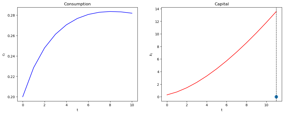
Evidently, our initial guess for \(\mu_0\) is too high, so initial consumption too low.
We know this because we miss our \(K_{T+1}=0\) target on the high side.
Now we automate things with a search-for-a-good \(\mu_0\) algorithm that stops when we hit the target \(K_{t+1} = 0\).
We use a bisection method.
We make an initial guess for \(C_0\) (we can eliminate \(\mu_0\) because \(C_0\) is an exact function of \(\mu_0\)).
We know that the lowest \(C_0\) can ever be is \(0\) and that the largest it can be is initial output \(f(K_0)\).
Guess \(C_0\) and shoot forward to \(T+1\).
If \(K_{T+1}>0\), we take it to be our new lower bound on \(C_0\).
If \(K_{T+1}<0\), we take it to be our new upper bound.
Make a new guess for \(C_0\) that is halfway between our new upper and lower bounds.
Shoot forward again, iterating on these steps until we converge.
When \(K_{T+1}\) gets close enough to \(0\) (i.e., within an error tolerance bounds), we stop.
@jit
def bisection(pp, c0, k0, T=10, tol=1e-4, max_iter=500, k_ter=0, verbose=True):

    # initial boundaries for guess c0
    c0_upper = pp.f(k0) + (1 - pp.δ) * k0
    c0_lower = 0

    i = 0
    while True:
        c_vec, k_vec = shooting(pp, c0, k0, T)
        error = k_vec[-1] - k_ter

        # check if the terminal condition is satisfied
        if np.abs(error) < tol:
            if verbose:
                print('Converged successfully on iteration ', i+1)
            return c_vec, k_vec

        i += 1
        if i == max_iter:
            if verbose:
                print('Convergence failed.')
            return c_vec, k_vec

        # if iteration continues, updates boundaries and guess of c0
        if error > 0:
            c0_lower = c0
        else:
            c0_upper = c0

        c0 = (c0_lower + c0_upper) / 2
def plot_paths(pp, c0, k0, T_arr, k_ter=0, k_ss=None, axs=None):

    if axs is None:
        fix, axs = plt.subplots(1, 3, figsize=(16, 4))
    ylabels = ['$c_t$', '$k_t$', r'$\mu_t$']
    titles = ['Consumption', 'Capital', 'Lagrange Multiplier']

    c_paths = []
    k_paths = []
    for T in T_arr:
        c_vec, k_vec = bisection(pp, c0, k0, T, k_ter=k_ter, verbose=False)
        c_paths.append(c_vec)
        k_paths.append(k_vec)

        μ_vec = pp.u_prime(c_vec)
        paths = [c_vec, k_vec, μ_vec]

        for i in range(3):
            axs[i].plot(paths[i])
            axs[i].set(xlabel='t', ylabel=ylabels[i], title=titles[i])

        # Plot steady state value of capital
        if k_ss is not None:
            axs[1].axhline(k_ss, c='k', ls='--', lw=1)

        axs[1].axvline(T+1, c='k', ls='--', lw=1)
        axs[1].scatter(T+1, paths[1][-1], s=80)

    return c_paths, k_paths
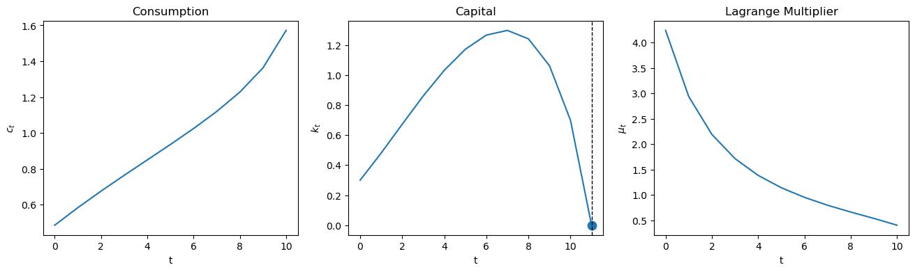
Now we can solve the model and plot the paths of consumption, capital, and Lagrange multiplier.
plot_paths(pp, 0.3, 0.3, [10]);
84.5. Setting Initial Capital to Steady State Capital#
When \(T \rightarrow +\infty\), the optimal allocation converges to steady state values of \(C_t\) and \(K_t\).
It is instructive to set \(K_0\) equal to the \(\lim_{T \rightarrow + \infty } K_t\), which we’ll call steady state capital.
In a steady state \(K_{t+1} = K_t=\bar{K}\) for all very large \(t\).
Evalauating feasibility constraint (84.5) at \(\bar K\) gives
Substituting \(K_t = \bar K\) and \(C_t=\bar C\) for all \(t\) into (84.14) gives
Defining \(\beta = \frac{1}{1+\rho}\), and cancelling gives
Simplifying gives
and
For production function (84.4), this becomes
As an example, after setting \(\alpha= .33\), \(\rho = 1/\beta-1 =1/(19/20)-1 = 20/19-19/19 = 1/19\), \(\delta = 1/50\), we get
Let’s verify this with Python and then use this steady state \(\bar K\) as our initial capital stock \(K_0\).
ρ = 1 / pp.β - 1
k_ss = pp.f_prime_inv(ρ+pp.δ)

print(f'steady state for capital is: {k_ss}')
steady state for capital is: 9.57583816331462
Now we plot
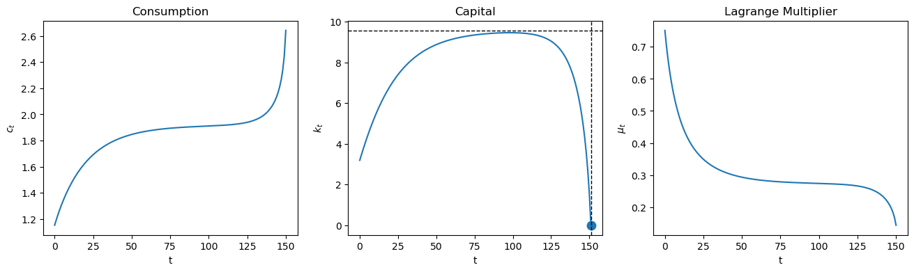
plot_paths(pp, 0.3, k_ss, [150], k_ss=k_ss);
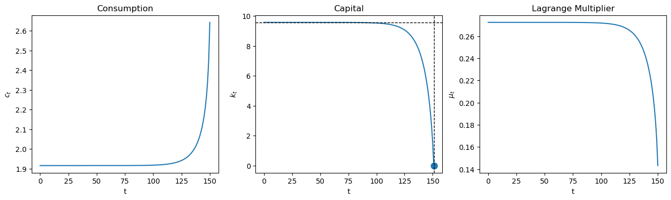
Evidently, with a large value of \(T\), \(K_t\) stays near \(K_0\) until \(t\) approaches \(T\) closely.
Let’s see what the planner does when we set \(K_0\) below \(\bar K\).
plot_paths(pp, 0.3, k_ss/3, [150], k_ss=k_ss);
Notice how the planner pushes capital toward the steady state, stays near there for a while, then pushes \(K_t\) toward the terminal value \(K_{T+1} =0\) when \(t\) closely approaches \(T\).
The following graphs compare optimal outcomes as we vary \(T\).
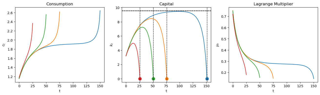
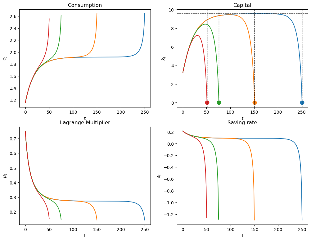
plot_paths(pp, 0.3, k_ss/3, [150, 75, 50, 25], k_ss=k_ss);
84.6. A Turnpike Property#
The following calculation indicates that when \(T\) is very large, the optimal capital stock stays close to its steady state value most of the time.
plot_paths(pp, 0.3, k_ss/3, [250, 150, 50, 25], k_ss=k_ss);
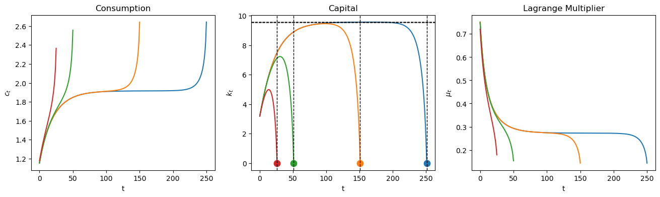
In the above graphs, different colors are associated with different horizons \(T\).
Notice that as the horizon increases, the planner keeps \(K_t\) closer to the steady state value \(\bar K\) for longer.
This pattern reflects a turnpike property of the steady state.
A rule of thumb for the planner is
from \(K_0\), push \(K_t\) toward the steady state and stay close to the steady state until time approaches \(T\).
The planner accomplishes this by adjusting the saving rate \(\frac{f(K_t) - C_t}{f(K_t)}\) over time.
Exercise 84.1
The turnpike property is independent of the initial condition \(K_0\) provided that \(T\) is sufficiently large.
Expand the plot_paths function so that it plots trajectories for multiple initial points using k0s = [k_ss*2, k_ss*3, k_ss/3].
Solution
Here is one solution
def plot_multiple_paths(pp, c0, k0s, T_arr, k_ter=0, k_ss=None, axs=None):
    if axs is None:
        fig, axs = plt.subplots(1, 3, figsize=(16, 4))

    ylabels = ['$c_t$', '$k_t$', r'$\mu_t$']
    titles = ['Consumption', 'Capital', 'Lagrange Multiplier']

    colors = plt.cm.viridis(np.linspace(0, 1, len(k0s)))

    all_c_paths = []
    all_k_paths = []

    for i, k0 in enumerate(k0s):
        k0_c_paths = []
        k0_k_paths = []

        for T in T_arr:
            c_vec, k_vec = bisection(pp, c0, k0, T, k_ter=k_ter, verbose=False)
            k0_c_paths.append(c_vec)
            k0_k_paths.append(k_vec)

            μ_vec = pp.u_prime(c_vec)
            paths = [c_vec, k_vec, μ_vec]

            for j in range(3):
                axs[j].plot(paths[j], color=colors[i],
                           label=f'$k_0 = {k0:.2f}$' if j == 0 and T == T_arr[0] else "", alpha=0.7)
                axs[j].set(xlabel='t', ylabel=ylabels[j], title=titles[j])

            if k_ss is not None and i == 0 and T == T_arr[0]:
                axs[1].axhline(k_ss, c='k', ls='--', lw=1)

            axs[1].axvline(T+1, c='k', ls='--', lw=1)
            axs[1].scatter(T+1, paths[1][-1], s=80, color=colors[i])

        all_c_paths.append(k0_c_paths)
        all_k_paths.append(k0_k_paths)

    # Add legend if multiple initial points
    if len(k0s) > 1:
        axs[0].legend()

    return all_c_paths, all_k_paths
_ = plot_multiple_paths(pp, 0.3, [k_ss*2, k_ss*3, k_ss/3], [250, 150, 75, 50], k_ss=k_ss)
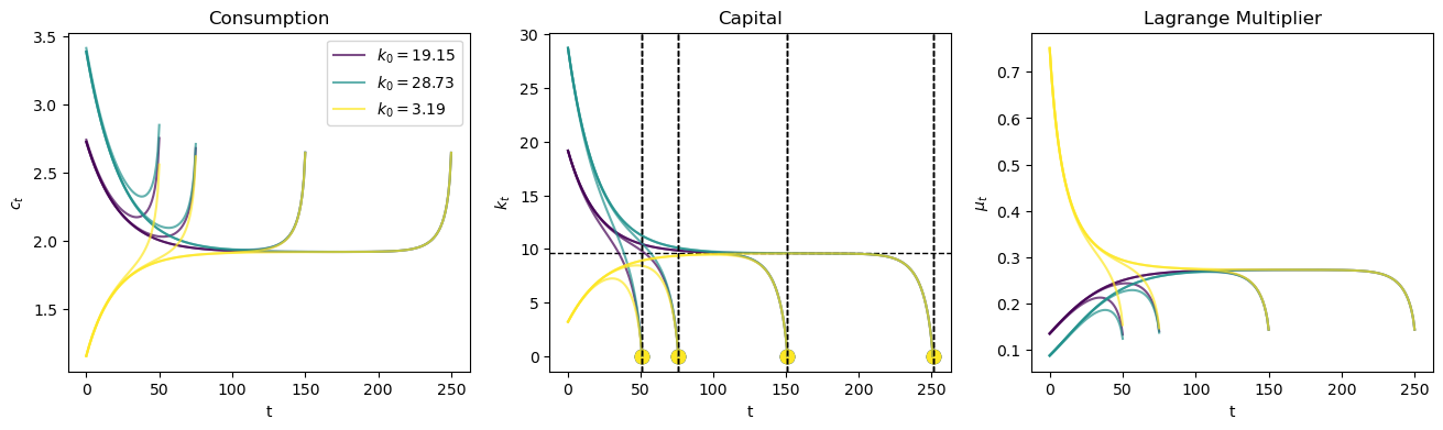
We see that the turnpike property holds for various initial values of \(K_0\).
Let’s calculate and plot the saving rate.
@jit
def saving_rate(pp, c_path, k_path):
    'Given paths of c and k, computes the path of saving rate.'
    production = pp.f(k_path[:-1])

    return (production - c_path) / production
def plot_saving_rate(pp, c0, k0, T_arr, k_ter=0, k_ss=None, s_ss=None):

    fix, axs = plt.subplots(2, 2, figsize=(12, 9))

    c_paths, k_paths = plot_paths(pp, c0, k0, T_arr, k_ter=k_ter, k_ss=k_ss, axs=axs.flatten())

    for i, T in enumerate(T_arr):
        s_path = saving_rate(pp, c_paths[i], k_paths[i])
        axs[1, 1].plot(s_path)

    axs[1, 1].set(xlabel='t', ylabel='$s_t$', title='Saving rate')

    if s_ss is not None:
        axs[1, 1].hlines(s_ss, 0, np.max(T_arr), linestyle='--')
plot_saving_rate(pp, 0.3, k_ss/3, [250, 150, 75, 50], k_ss=k_ss)
84.7. A Limiting Infinite Horizon Economy#
We want to set \(T = +\infty\).
The appropriate thing to do is to replace terminal condition (84.12) with
a condition that will be satisfied by a path that converges to an optimal steady state.
We can approximate the optimal path by starting from an arbitrary initial \(K_0\) and shooting towards the optimal steady state \(K\) at a large but finite \(T+1\).
In the following code, we do this for a large \(T\) and plot consumption, capital, and the saving rate.
We know that in the steady state that the saving rate is constant and that \(\bar s= \frac{f(\bar K)-\bar C}{f(\bar K)}\).
From (84.17) the steady state saving rate equals
The steady state saving rate \(\bar S = \bar s f(\bar K)\) is the amount required to offset capital depreciation each period.
We first study optimal capital paths that start below the steady state.
# steady state of saving rate
s_ss = pp.δ * k_ss / pp.f(k_ss)

plot_saving_rate(pp, 0.3, k_ss/3, [130], k_ter=k_ss, k_ss=k_ss, s_ss=s_ss)
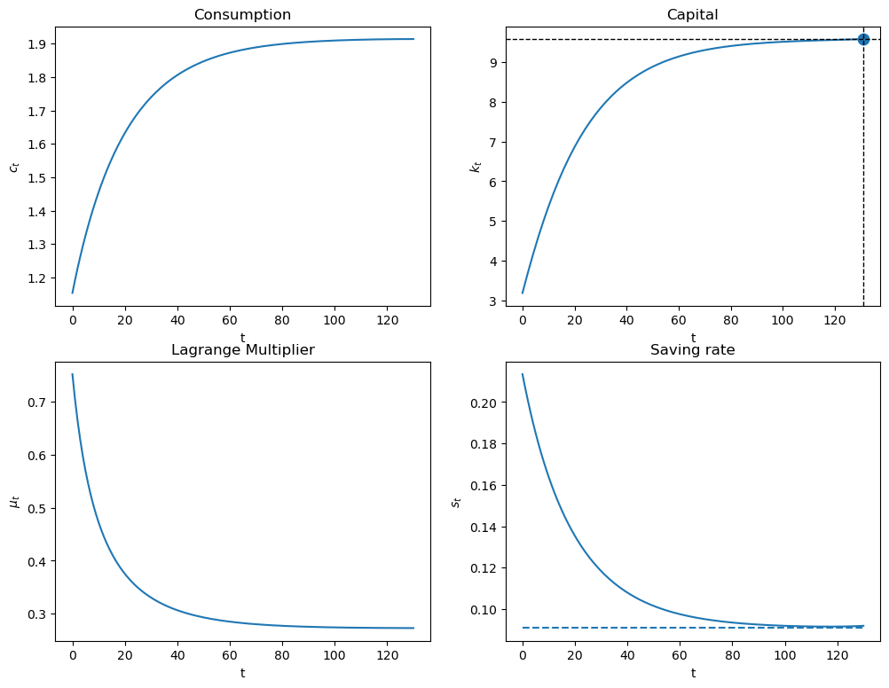
Since \(K_0<\bar K\), \(f'(K_0)>\rho +\delta\).
The planner chooses a positive saving rate that is higher than the steady state saving rate.
Note that \(f''(K)<0\), so as \(K\) rises, \(f'(K)\) declines.
The planner slowly lowers the saving rate until reaching a steady state in which \(f'(K)=\rho +\delta\).
84.8. Stable Manifold and Phase Diagram#
We now describe a classic diagram that describes an optimal \((K_{t+1}, C_t)\) path.
The diagram has \(K\) on the ordinate axis and \(C\) on the coordinate axis.
Given an arbitrary and fixed \(K\), a fixed point \(C\) of the consumption Euler equation (84.15) satisfies
which implies
A positive fixed point \(C = \tilde C(K)\) exists only if \(f\left(K\right)+\left(1-\delta\right)K-f^{\prime-1}\left(\frac{1}{\beta}-\left(1-\delta\right)\right)>0\)
@jit
def C_tilde(K, pp):

    return pp.f(K) + (1 - pp.δ) * K - pp.f_prime_inv(1 / pp.β - 1 + pp.δ)
Next note that given a time-invariant arbitrary \(C\), a fixed point \(K\) of the feasibility condition (84.5) solves the following equation
A fixed point of the above equation is described by a function
@jit
def K_diff(K, C, pp):
    return pp.f(K) - pp.δ * K - C

@jit
def K_tilde(C, pp):

    res = brentq(K_diff, 1e-6, 100, args=(C, pp))

    return res.root
A steady state \(\left(K_s, C_s\right)\) is a pair \((K,C)\) that satisfies both equations (84.18) and (84.19).
It is thus the intersection of the two curves \(\tilde{C}\) and \(\tilde{K}\) that we’ll plot in Figure Fig. 84.1 below.
We can compute \(K_s\) by solving the equation \(K_s = \tilde{K}\left(\tilde{C}\left(K_s\right)\right)\)
@jit
def K_tilde_diff(K, pp):

    K_out = K_tilde(C_tilde(K, pp), pp)

    return K - K_out
res = brentq(K_tilde_diff, 8, 10, args=(pp,))

Ks = res.root
Cs = C_tilde(Ks, pp)

Ks, Cs
(9.575838163314447, 1.9160839808123402)
We can use the shooting algorithm to compute trajectories that approach \(\left(K_s, C_s\right)\).
For a given \(K\), let’s compute \(\vec{C}\) and \(\vec{K}\) for a large \(T\) , e.g., \(=200\).
We compute \(C_0\) by the bisection algorithm that assures that \(K_T=K_s\).
Let’s compute two trajectories towards \(\left(K_s, C_s\right)\) that start from different sides of \(K_s\): \(\bar{K}_0=1e-3<K_s<\bar{K}_1=15\).
c_vec1, k_vec1 = bisection(pp, 5, 15, T=200, k_ter=Ks)
c_vec2, k_vec2 = bisection(pp, 1e-3, 1e-3, T=200, k_ter=Ks)
Converged successfully on iteration  46
Converged successfully on iteration  51
The following code generates Figure Fig. 84.1, which is patterned on a graph that appears on page 411 of [Intriligator, 2002].
Figure Fig. 84.1 is a classic “phase plane” with “state” variable \(K\) on the ordinate axis and “co-state” variable \(C\) on the coordinate axis.
Figure Fig. 84.1 plots three curves:
the blue line graphs \(C = \tilde C (K)\) of fixed points described by equation (84.18).
the red line graphs \(K = \tilde K(C)\) of fixed points described by equation (84.19)
the green line graphs the stable traced out by paths that converge to the steady state starting from an arbitrary \(K_0\) at time \(0\).
for a given \(K_0\), the shooting algorithm sets \(C_0\) to the coordinate on the green line in order to initiate a path that converges to the optimal steady state
the arrows on the green line show the direction in which dynamics (84.16) push successive \((K_{t+1}, C_t)\) pairs.
In addition to the three curves, Figure Fig. 84.1 plots arrows that point where the dynamics (84.16) drive the system when, for a given \(K_0\), \(C_0\) is not on the stable manifold depicted in the green line.
If \(C_0\) is set below the green line for a given \(K_0\), too much capital is accumulated
If \(C_0\) is set above the green line for a given \(K_0\), too little capital is accumulated
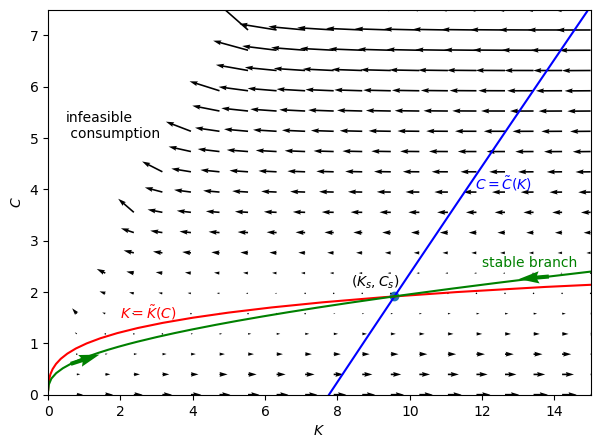
Fig. 84.1 Stable Manifold and Phase Plane#
84.9. Concluding Remarks#
In Cass-Koopmans Competitive Equilibrium, we study a decentralized version of an economy with exactly the same technology and preference structure as deployed here.
In that lecture, we replace the planner of this lecture with Adam Smith’s invisible hand.
In place of quantity choices made by the planner, there are market prices that are set by a deus ex machina from outside the model, a so-called invisible hand.
Equilibrium market prices must reconcile distinct decisions that are made independently by a representative household and a representative firm.
The relationship between a command economy like the one studied in this lecture and a market economy like that studied in Cass-Koopmans Competitive Equilibrium is a foundational topic in general equilibrium theory and welfare economics.
84.9.1. Exercise#
Exercise 84.2
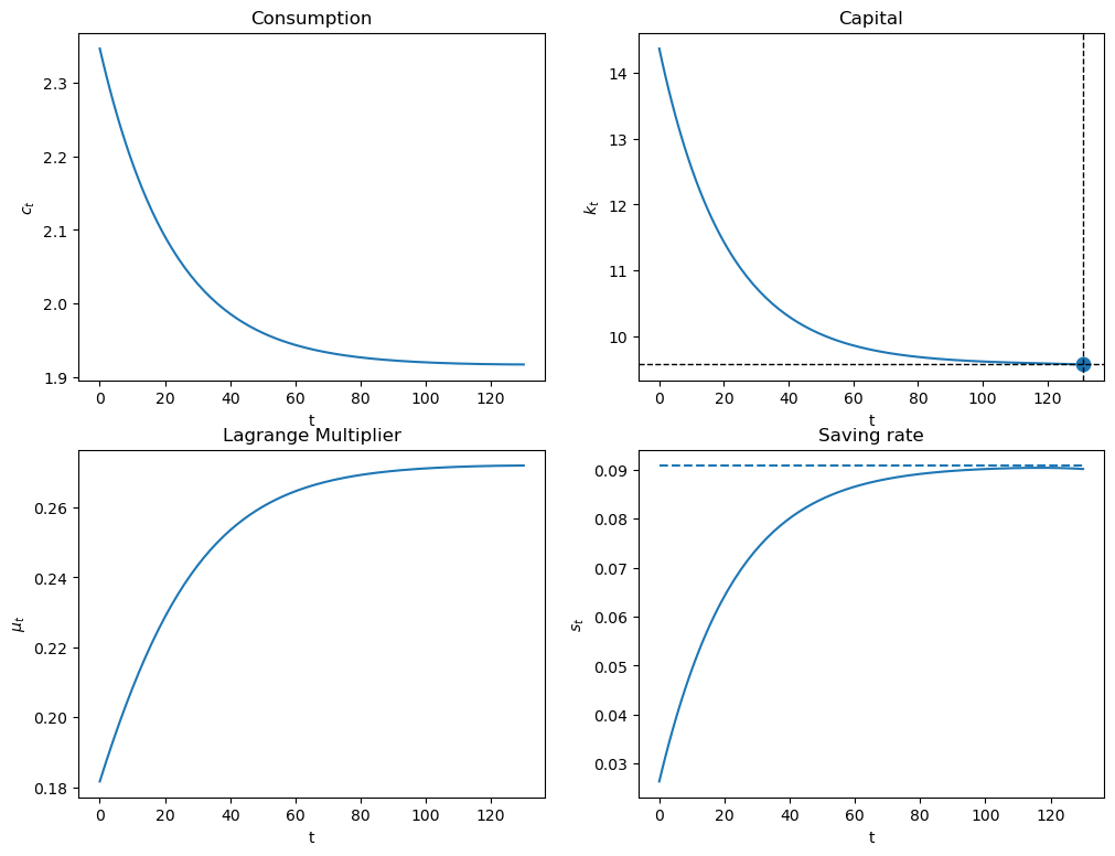
Plot the optimal consumption, capital, and saving paths when the initial capital level begins at 1.5 times the steady state level as we shoot towards the steady state at \(T=130\).
Why does the saving rate respond as it does?
Solution
plot_saving_rate(pp, 0.3, k_ss*1.5, [130], k_ter=k_ss, k_ss=k_ss, s_ss=s_ss)