24. Finite Markov Chains #

Contents

Finite Markov Chains

In addition to what’s in Anaconda, this lecture will need the following libraries:

!pip install quantecon

24.1. Overview #

Markov chains are one of the most useful classes of stochastic processes, being

simple, flexible and supported by many elegant theoretical results
valuable for building intuition about random dynamic models
central to quantitative modeling in their own right

You will find them in many of the workhorse models of economics and finance.

In this lecture, we review some of the theory of Markov chains.

We will also introduce some of the high-quality routines for working with Markov chains available in QuantEcon.py.

Prerequisite knowledge is basic probability and linear algebra.

Let’s start with some standard imports:

import matplotlib.pyplot as plt
plt.rcParams["figure.figsize"] = (11, 5)  #set default figure size
import quantecon as qe
import numpy as np
from mpl_toolkits.mplot3d import Axes3D

24.2. Definitions #

The following concepts are fundamental.

24.2.1. Stochastic Matrices#

A stochastic matrix (or Markov matrix) is an \(n \times n\) square matrix \(P\) such that

each element of \(P\) is nonnegative, and
each row of \(P\) sums to one

Each row of \(P\) can be regarded as a probability mass function over \(n\) possible outcomes.

It is too not difficult to check 1 that if \(P\) is a stochastic matrix, then so is the \(k\)-th power \(P^k\) for all \(k \in \mathbb N\).

24.2.2. Markov Chains#

There is a close connection between stochastic matrices and Markov chains.

To begin, let \(S\) be a finite set with \(n\) elements \(\{x_1, \ldots, x_n\}\).

The set \(S\) is called the state space and \(x_1, \ldots, x_n\) are the state values.

A Markov chain \(\{X_t\}\) on \(S\) is a sequence of random variables on \(S\) that have the Markov property.

This means that, for any date \(t\) and any state \(y \in S\),

(24.1)#\[\mathbb P \{ X_{t+1} = y \,|\, X_t \} = \mathbb P \{ X_{t+1} = y \,|\, X_t, X_{t-1}, \ldots \}\]

In other words, knowing the current state is enough to know probabilities for future states.

In particular, the dynamics of a Markov chain are fully determined by the set of values

(24.2)#\[P(x, y) := \mathbb P \{ X_{t+1} = y \,|\, X_t = x \} \qquad (x, y \in S)\]

By construction,

\(P(x, y)\) is the probability of going from \(x\) to \(y\) in one unit of time (one step)
\(P(x, \cdot)\) is the conditional distribution of \(X_{t+1}\) given \(X_t = x\)

We can view \(P\) as a stochastic matrix where

\[ P_{ij} = P(x_i, x_j) \qquad 1 \leq i, j \leq n \]

Going the other way, if we take a stochastic matrix \(P\), we can generate a Markov chain \(\{X_t\}\) as follows:

draw \(X_0\) from a marginal distribution \(\psi\)
for each \(t = 0, 1, \ldots\), draw \(X_{t+1}\) from \(P(X_t,\cdot)\)

By construction, the resulting process satisfies (24.2).

24.2.3. Example 1#

Consider a worker who, at any given time \(t\), is either unemployed (state 0) or employed (state 1).

Suppose that, over a one month period,

An unemployed worker finds a job with probability \(\alpha \in (0, 1)\).
An employed worker loses her job and becomes unemployed with probability \(\beta \in (0, 1)\).

In terms of a Markov model, we have

\(S = \{ 0, 1\}\)
\(P(0, 1) = \alpha\) and \(P(1, 0) = \beta\)

We can write out the transition probabilities in matrix form as

(24.3)#\[\begin{split}P = \left( \begin{array}{cc} 1 - \alpha & \alpha \\ \beta & 1 - \beta \end{array} \right)\end{split}\]

Once we have the values \(\alpha\) and \(\beta\), we can address a range of questions, such as

What is the average duration of unemployment?
Over the long-run, what fraction of time does a worker find herself unemployed?
Conditional on employment, what is the probability of becoming unemployed at least once over the next 12 months?

We’ll cover such applications below.

24.2.4. Example 2#

From US unemployment data, Hamilton [Hamilton, 2005] estimated the stochastic matrix

\[\begin{split} P = \left( \begin{array}{ccc} 0.971 & 0.029 & 0 \\ 0.145 & 0.778 & 0.077 \\ 0 & 0.508 & 0.492 \end{array} \right) \end{split}\]

where

the frequency is monthly
the first state represents “normal growth”
the second state represents “mild recession”
the third state represents “severe recession”

For example, the matrix tells us that when the state is normal growth, the state will again be normal growth next month with probability 0.97.

In general, large values on the main diagonal indicate persistence in the process \(\{ X_t \}\).

This Markov process can also be represented as a directed graph, with edges labeled by transition probabilities

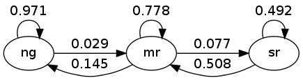
Here “ng” is normal growth, “mr” is mild recession, etc.

24.3. Simulation #

One natural way to answer questions about Markov chains is to simulate them.

(To approximate the probability of event \(E\), we can simulate many times and count the fraction of times that \(E\) occurs).

Nice functionality for simulating Markov chains exists in QuantEcon.py.

Efficient, bundled with lots of other useful routines for handling Markov chains.

However, it’s also a good exercise to roll our own routines — let’s do that first and then come back to the methods in QuantEcon.py.

In these exercises, we’ll take the state space to be \(S = 0,\ldots, n-1\).

24.3.1. Rolling Our Own#

To simulate a Markov chain, we need its stochastic matrix \(P\) and a marginal probability distribution \(\psi\) from which to draw a realization of \(X_0\).

The Markov chain is then constructed as discussed above. To repeat:

At time \(t=0\), draw a realization of \(X_0\) from \(\psi\).
At each subsequent time \(t\), draw a realization of the new state \(X_{t+1}\) from \(P(X_t, \cdot)\).

To implement this simulation procedure, we need a method for generating draws from a discrete distribution.

For this task, we’ll use random.draw from QuantEcon, which works as follows:

ψ = (0.3, 0.7)           # probabilities over {0, 1}
cdf = np.cumsum(ψ)       # convert into cummulative distribution
qe.random.draw(cdf, 5)   # generate 5 independent draws from ψ

array([1, 1, 0, 0, 1])

We’ll write our code as a function that accepts the following three arguments

A stochastic matrix P
An initial state init
A positive integer sample_size representing the length of the time series the function should return

def mc_sample_path(P, ψ_0=None, sample_size=1_000):

    # set up
    P = np.asarray(P)
    X = np.empty(sample_size, dtype=int)

    # Convert each row of P into a cdf
    n = len(P)
    P_dist = [np.cumsum(P[i, :]) for i in range(n)]

    # draw initial state, defaulting to 0
    if ψ_0 is not None:
        X_0 = qe.random.draw(np.cumsum(ψ_0))
    else:
        X_0 = 0

    # simulate
    X[0] = X_0
    for t in range(sample_size - 1):
        X[t+1] = qe.random.draw(P_dist[X[t]])

    return X

Let’s see how it works using the small matrix

P = [[0.4, 0.6],
     [0.2, 0.8]]

As we’ll see later, for a long series drawn from P, the fraction of the sample that takes value 0 will be about 0.25.

Moreover, this is true, regardless of the initial distribution from which \(X_0\) is drawn.

The following code illustrates this

X = mc_sample_path(P, ψ_0=[0.1, 0.9], sample_size=100_000)
np.mean(X == 0)

0.25126

You can try changing the initial distribution to confirm that the output is always close to 0.25, at least for the P matrix above.

24.3.2. Using QuantEcon’s Routines#

As discussed above, QuantEcon.py has routines for handling Markov chains, including simulation.

Here’s an illustration using the same P as the preceding example

from quantecon import MarkovChain

mc = qe.MarkovChain(P)
X = mc.simulate(ts_length=1_000_000)
np.mean(X == 0)

0.250275

The QuantEcon.py routine is JIT compiled and much faster.

%time mc_sample_path(P, sample_size=1_000_000) # Our homemade code version

CPU times: user 1.28 s, sys: 0 ns, total: 1.28 s
Wall time: 1.28 s

array([0, 1, 1, ..., 0, 1, 1])

%time mc.simulate(ts_length=1_000_000) # qe code version

CPU times: user 23.5 ms, sys: 339 µs, total: 23.9 ms
Wall time: 23.6 ms

array([1, 1, 1, ..., 1, 0, 1])

24.3.2.1. Adding State Values and Initial Conditions#

If we wish to, we can provide a specification of state values to MarkovChain.

These state values can be integers, floats, or even strings.

The following code illustrates

mc = qe.MarkovChain(P, state_values=('unemployed', 'employed'))
mc.simulate(ts_length=4, init='employed')

array(['employed', 'employed', 'employed', 'employed'], dtype='<U10')

mc.simulate(ts_length=4, init='unemployed')

array(['unemployed', 'unemployed', 'unemployed', 'employed'], dtype='<U10')

mc.simulate(ts_length=4)  # Start at randomly chosen initial state

array(['employed', 'employed', 'employed', 'employed'], dtype='<U10')

If we want to see indices rather than state values as outputs as we can use

mc.simulate_indices(ts_length=4)

array([0, 0, 1, 1])

24.4. Marginal Distributions #

Suppose that

\(\{X_t\}\) is a Markov chain with stochastic matrix \(P\)
the marginal distribution of \(X_t\) is known to be \(\psi_t\)

What then is the marginal distribution of \(X_{t+1}\), or, more generally, of \(X_{t+m}\)?

To answer this, we let \(\psi_t\) be the marginal distribution of \(X_t\) for \(t = 0, 1, 2, \ldots\).

Our first aim is to find \(\psi_{t + 1}\) given \(\psi_t\) and \(P\).

To begin, pick any \(y \in S\).

Using the law of total probability, we can decompose the probability that \(X_{t+1} = y\) as follows:

\[ \mathbb P \{X_{t+1} = y \} = \sum_{x \in S} \mathbb P \{ X_{t+1} = y \, | \, X_t = x \} \cdot \mathbb P \{ X_t = x \} \]

In words, to get the probability of being at \(y\) tomorrow, we account for all ways this can happen and sum their probabilities.

Rewriting this statement in terms of marginal and conditional probabilities gives

\[ \psi_{t+1}(y) = \sum_{x \in S} P(x,y) \psi_t(x) \]

There are \(n\) such equations, one for each \(y \in S\).

If we think of \(\psi_{t+1}\) and \(\psi_t\) as row vectors, these \(n\) equations are summarized by the matrix expression

(24.4)#\[\psi_{t+1} = \psi_t P\]

Thus, to move a marginal distribution forward one unit of time, we postmultiply by \(P\).

By postmultiplying \(m\) times, we move a marginal distribution forward \(m\) steps into the future.

Hence, iterating on (24.4), the expression \(\psi_{t+m} = \psi_t P^m\) is also valid — here \(P^m\) is the \(m\)-th power of \(P\).

As a special case, we see that if \(\psi_0\) is the initial distribution from which \(X_0\) is drawn, then \(\psi_0 P^m\) is the distribution of \(X_m\).

This is very important, so let’s repeat it

(24.5)#\[X_0 \sim \psi_0 \quad \implies \quad X_m \sim \psi_0 P^m\]

and, more generally,

(24.6)#\[X_t \sim \psi_t \quad \implies \quad X_{t+m} \sim \psi_t P^m\]

24.4.1. Multiple Step Transition Probabilities#

We know that the probability of transitioning from \(x\) to \(y\) in one step is \(P(x,y)\).

It turns out that the probability of transitioning from \(x\) to \(y\) in \(m\) steps is \(P^m(x,y)\), the \((x,y)\)-th element of the \(m\)-th power of \(P\).

To see why, consider again (24.6), but now with a \(\psi_t\) that puts all probability on state \(x\) so that the transition probabilities are

1 in the \(x\)-th position and zero elsewhere

Inserting this into (24.6), we see that, conditional on \(X_t = x\), the distribution of \(X_{t+m}\) is the \(x\)-th row of \(P^m\).

In particular

\[ \mathbb P \{X_{t+m} = y \,|\, X_t = x \} = P^m(x, y) = (x, y) \text{-th element of } P^m \]

24.4.2. Example: Probability of Recession#

Recall the stochastic matrix \(P\) for recession and growth considered above.

Suppose that the current state is unknown — perhaps statistics are available only at the end of the current month.

We guess that the probability that the economy is in state \(x\) is \(\psi(x)\).

The probability of being in recession (either mild or severe) in 6 months time is given by the inner product

\[\begin{split} \psi P^6 \cdot \left( \begin{array}{c} 0 \\ 1 \\ 1 \end{array} \right) \end{split}\]

24.4.3. Example 2: Cross-Sectional Distributions#

The marginal distributions we have been studying can be viewed either as probabilities or as cross-sectional frequencies that a Law of Large Numbers leads us to anticipate for large samples.

To illustrate, recall our model of employment/unemployment dynamics for a given worker discussed above.

Consider a large population of workers, each of whose lifetime experience is described by the specified dynamics, with each worker’s outcomes being realizations of processes that are statistically independent of all other workers’ processes.

Let \(\psi\) be the current cross-sectional distribution over \(\{ 0, 1 \}\).

The cross-sectional distribution records fractions of workers employed and unemployed at a given moment.

For example, \(\psi(0)\) is the unemployment rate.

What will the cross-sectional distribution be in 10 periods hence?

The answer is \(\psi P^{10}\), where \(P\) is the stochastic matrix in (24.3).

This is because each worker’s state evolves according to \(P\), so \(\psi P^{10}\) is a marginal distibution for a single randomly selected worker.

But when the sample is large, outcomes and probabilities are roughly equal (by an application of the Law of Large Numbers).

So for a very large (tending to infinite) population, \(\psi P^{10}\) also represents fractions of workers in each state.

This is exactly the cross-sectional distribution.

24.5. Irreducibility and Aperiodicity #

Irreducibility and aperiodicity are central concepts of modern Markov chain theory.

Let’s see what they’re about.

24.5.1. Irreducibility#

Let \(P\) be a fixed stochastic matrix.

Two states \(x\) and \(y\) are said to communicate with each other if there exist positive integers \(j\) and \(k\) such that

\[ P^j(x, y) > 0 \quad \text{and} \quad P^k(y, x) > 0 \]

In view of our discussion above, this means precisely that

state \(x\) can eventually be reached from state \(y\), and
state \(y\) can eventually be reached from state \(x\)

The stochastic matrix \(P\) is called irreducible if all states communicate; that is, if \(x\) and \(y\) communicate for all \((x, y)\) in \(S \times S\).

For example, consider the following transition probabilities for wealth of a fictitious set of households

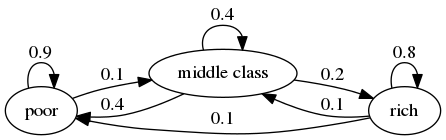
We can translate this into a stochastic matrix, putting zeros where there’s no edge between nodes

\[\begin{split} P := \left( \begin{array}{ccc} 0.9 & 0.1 & 0 \\ 0.4 & 0.4 & 0.2 \\ 0.1 & 0.1 & 0.8 \end{array} \right) \end{split}\]

It’s clear from the graph that this stochastic matrix is irreducible: we can eventually reach any state from any other state.

We can also test this using QuantEcon.py’s MarkovChain class

P = [[0.9, 0.1, 0.0],
     [0.4, 0.4, 0.2],
     [0.1, 0.1, 0.8]]

mc = qe.MarkovChain(P, ('poor', 'middle', 'rich'))
mc.is_irreducible

True

Here’s a more pessimistic scenario in which poor people remain poor forever

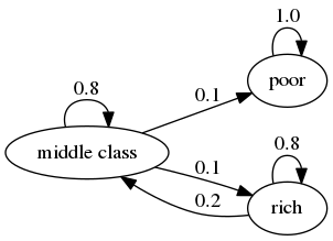
This stochastic matrix is not irreducible, since, for example, rich is not accessible from poor.

Let’s confirm this

P = [[1.0, 0.0, 0.0],
     [0.1, 0.8, 0.1],
     [0.0, 0.2, 0.8]]

mc = qe.MarkovChain(P, ('poor', 'middle', 'rich'))
mc.is_irreducible

False

We can also determine the “communication classes”

mc.communication_classes

[array(['poor'], dtype='<U6'), array(['middle', 'rich'], dtype='<U6')]

It might be clear to you already that irreducibility is going to be important in terms of long run outcomes.

For example, poverty is a life sentence in the second graph but not the first.

We’ll come back to this a bit later.

24.5.2. Aperiodicity#

Loosely speaking, a Markov chain is called periodic if it cycles in a predictable way, and aperiodic otherwise.

Here’s a trivial example with three states

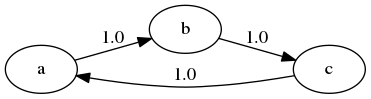
The chain cycles with period 3:

P = [[0, 1, 0],
     [0, 0, 1],
     [1, 0, 0]]

mc = qe.MarkovChain(P)
mc.period

More formally, the period of a state \(x\) is the largest common divisor of a set of integers

\[ D(x) := \{j \geq 1 : P^j(x, x) > 0\} \]

In the last example, \(D(x) = \{3, 6, 9, \ldots\}\) for every state \(x\), so the period is 3.

A stochastic matrix is called aperiodic if the period of every state is 1, and periodic otherwise.

For example, the stochastic matrix associated with the transition probabilities below is periodic because, for example, state \(a\) has period 2

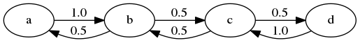
We can confirm that the stochastic matrix is periodic with the following code

P = [[0.0, 1.0, 0.0, 0.0],
     [0.5, 0.0, 0.5, 0.0],
     [0.0, 0.5, 0.0, 0.5],
     [0.0, 0.0, 1.0, 0.0]]

mc = qe.MarkovChain(P)
mc.period

mc.is_aperiodic

False

24.6. Stationary Distributions #

As seen in (24.4), we can shift a marginal distribution forward one unit of time via postmultiplication by \(P\).

Some distributions are invariant under this updating process — for example,

P = np.array([[0.4, 0.6],
              [0.2, 0.8]])
ψ = (0.25, 0.75)
ψ @ P

array([0.25, 0.75])

Such distributions are called stationary or invariant.

Formally, a marginal distribution \(\psi^*\) on \(S\) is called stationary for \(P\) if \(\psi^* = \psi^* P\).

(This is the same notion of stationarity that we learned about in the lecture on AR(1) processes applied to a different setting.)

From this equality, we immediately get \(\psi^* = \psi^* P^t\) for all \(t\).

This tells us an important fact: If the distribution of \(X_0\) is a stationary distribution, then \(X_t\) will have this same distribution for all \(t\).

Hence stationary distributions have a natural interpretation as stochastic steady states — we’ll discuss this more soon.

Mathematically, a stationary distribution is a fixed point of \(P\) when \(P\) is thought of as the map \(\psi \mapsto \psi P\) from (row) vectors to (row) vectors.

Theorem. Every stochastic matrix \(P\) has at least one stationary distribution.

(We are assuming here that the state space \(S\) is finite; if not more assumptions are required)

For proof of this result, you can apply Brouwer’s fixed point theorem, or see EDTC, theorem 4.3.5.

There can be many stationary distributions corresponding to a given stochastic matrix \(P\).

For example, if \(P\) is the identity matrix, then all marginal distributions are stationary.

To get uniqueness an invariant distribution, the transition matrix \(P\) must have the property that no nontrivial subsets of the state space are infinitely persistent.

A subset of the state space is infinitely persistent if other parts of the state space cannot be accessed from it.

Thus, infinite persistence of a non-trivial subset is the opposite of irreducibility.

This gives some intuition for the following fundamental theorem.

Theorem. If \(P\) is both aperiodic and irreducible, then

\(P\) has exactly one stationary distribution \(\psi^*\).
For any initial marginal distribution \(\psi_0\), we have \(\| \psi_0 P^t - \psi^* \| \to 0\) as \(t \to \infty\).

For a proof, see, for example, theorem 5.2 of [Häggström, 2002].

(Note that part 1 of the theorem only requires irreducibility, whereas part 2 requires both irreducibility and aperiodicity)

A stochastic matrix that satisfies the conditions of the theorem is sometimes called uniformly ergodic.

A sufficient condition for aperiodicity and irreducibility is that every element of \(P\) is strictly positive.

Try to convince yourself of this.

24.6.1. Example#

Recall our model of the employment/unemployment dynamics of a particular worker discussed above.

Assuming \(\alpha \in (0,1)\) and \(\beta \in (0,1)\), the uniform ergodicity condition is satisfied.

Let \(\psi^* = (p, 1-p)\) be the stationary distribution, so that \(p\) corresponds to unemployment (state 0).

Using \(\psi^* = \psi^* P\) and a bit of algebra yields

\[ p = \frac{\beta}{\alpha + \beta} \]

This is, in some sense, a steady state probability of unemployment — more about the interpretation of this below.

Not surprisingly it tends to zero as \(\beta \to 0\), and to one as \(\alpha \to 0\).

24.6.2. Calculating Stationary Distributions#

As discussed above, a particular Markov matrix \(P\) can have many stationary distributions.

That is, there can be many row vectors \(\psi\) such that \(\psi = \psi P\).

In fact if \(P\) has two distinct stationary distributions \(\psi_1, \psi_2\) then it has infinitely many, since in this case, as you can verify, for any \(\lambda \in [0, 1]\)

\[ \psi_3 := \lambda \psi_1 + (1 - \lambda) \psi_2 \]

is a stationary distribution for \(P\).

If we restrict attention to the case in which only one stationary distribution exists, one way to finding it is to solve the system

(24.7)#\[ \psi (I_n - P) = 0 \]

for \(\psi\), where \(I_n\) is the \(n \times n\) identity.

But the zero vector solves system (24.7), so we must proceed cautiously.

We want to impose the restriction that \(\psi\) is a probability distribution.

There are various ways to do this.

One option is to regard solving system (24.7) as an eigenvector problem: a vector \(\psi\) such that \(\psi = \psi P\) is a left eigenvector associated with the unit eigenvalue \(\lambda = 1\).

A stable and sophisticated algorithm specialized for stochastic matrices is implemented in QuantEcon.py.

This is the one we recommend:

P = [[0.4, 0.6],
     [0.2, 0.8]]

mc = qe.MarkovChain(P)
mc.stationary_distributions  # Show all stationary distributions

array([[0.25, 0.75]])

24.6.3. Convergence to Stationarity#

Part 2 of the Markov chain convergence theorem stated above tells us that the marginal distribution of \(X_t\) converges to the stationary distribution regardless of where we begin.

This adds considerable authority to our interpretation of \(\psi^*\) as a stochastic steady state.

The convergence in the theorem is illustrated in the next figure

P = ((0.971, 0.029, 0.000),
     (0.145, 0.778, 0.077),
     (0.000, 0.508, 0.492))
P = np.array(P)

ψ = (0.0, 0.2, 0.8)        # Initial condition

fig = plt.figure(figsize=(8, 6))
ax = fig.add_subplot(111, projection='3d')

ax.set(xlim=(0, 1), ylim=(0, 1), zlim=(0, 1),
       xticks=(0.25, 0.5, 0.75),
       yticks=(0.25, 0.5, 0.75),
       zticks=(0.25, 0.5, 0.75))

x_vals, y_vals, z_vals = [], [], []
for t in range(20):
    x_vals.append(ψ[0])
    y_vals.append(ψ[1])
    z_vals.append(ψ[2])
    ψ = ψ @ P

ax.scatter(x_vals, y_vals, z_vals, c='r', s=60)
ax.view_init(30, 210)

mc = qe.MarkovChain(P)
ψ_star = mc.stationary_distributions[0]
ax.scatter(ψ_star[0], ψ_star[1], ψ_star[2], c='k', s=60)

plt.show()

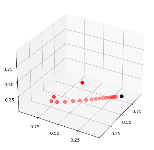
_images/c637beb99372e3cb2f1180415d51233fe39d57a4761a0635281664c3a226e0f6.png

Here

\(P\) is the stochastic matrix for recession and growth considered above.
The highest red dot is an arbitrarily chosen initial marginal probability distribution \(\psi\), represented as a vector in \(\mathbb R^3\).
The other red dots are the marginal distributions \(\psi P^t\) for \(t = 1, 2, \ldots\).
The black dot is \(\psi^*\).

You might like to try experimenting with different initial conditions.

24.7. Ergodicity #

Under irreducibility, yet another important result obtains: for all \(x \in S\),

(24.8)#\[\frac{1}{m} \sum_{t = 1}^m \mathbf{1}\{X_t = x\} \to \psi^*(x) \quad \text{as } m \to \infty\]

Here

\(\mathbf{1}\{X_t = x\} = 1\) if \(X_t = x\) and zero otherwise
convergence is with probability one
the result does not depend on the marginal distribution of \(X_0\)

The result tells us that the fraction of time the chain spends at state \(x\) converges to \(\psi^*(x)\) as time goes to infinity.

This gives us another way to interpret the stationary distribution — provided that the convergence result in (24.8) is valid.

The convergence asserted in (24.8) is a special case of a law of large numbers result for Markov chains — see EDTC, section 4.3.4 for some additional information.

24.7.1. Example#

Recall our cross-sectional interpretation of the employment/unemployment model discussed above.

Assume that \(\alpha \in (0,1)\) and \(\beta \in (0,1)\), so that irreducibility and aperiodicity both hold.

We saw that the stationary distribution is \((p, 1-p)\), where

\[ p = \frac{\beta}{\alpha + \beta} \]

In the cross-sectional interpretation, this is the fraction of people unemployed.

In view of our latest (ergodicity) result, it is also the fraction of time that a single worker can expect to spend unemployed.

Thus, in the long-run, cross-sectional averages for a population and time-series averages for a given person coincide.

This is one aspect of the concept of ergodicity.

24.8. Computing Expectations #

We sometimes want to compute mathematical expectations of functions of \(X_t\) of the form

(24.9)#\[\mathbb E [ h(X_t) ]\]

and conditional expectations such as

(24.10)#\[\mathbb E [ h(X_{t + k}) \mid X_t = x]\]

where

\(\{X_t\}\) is a Markov chain generated by \(n \times n\) stochastic matrix \(P\)
\(h\) is a given function, which, in terms of matrix algebra, we’ll think of as the column vector

\[\begin{split} h = \left( \begin{array}{c} h(x_1) \\ \vdots \\ h(x_n) \end{array} \right) \end{split}\]

Computing the unconditional expectation (24.9) is easy.

We just sum over the marginal distribution of \(X_t\) to get

\[ \mathbb E [ h(X_t) ] = \sum_{x \in S} (\psi P^t)(x) h(x) \]

Here \(\psi\) is the distribution of \(X_0\).

Since \(\psi\) and hence \(\psi P^t\) are row vectors, we can also write this as

\[ \mathbb E [ h(X_t) ] = \psi P^t h \]

For the conditional expectation (24.10), we need to sum over the conditional distribution of \(X_{t + k}\) given \(X_t = x\).

We already know that this is \(P^k(x, \cdot)\), so

(24.11)#\[\mathbb E [ h(X_{t + k}) \mid X_t = x] = (P^k h)(x)\]

The vector \(P^k h\) stores the conditional expectation \(\mathbb E [ h(X_{t + k}) \mid X_t = x]\) over all \(x\).

24.8.1. Iterated Expectations#

The law of iterated expectations states that

\[ \mathbb E \left[ \mathbb E [ h(X_{t + k}) \mid X_t = x] \right] = \mathbb E [ h(X_{t + k}) ] \]

where the outer \( \mathbb E\) on the left side is an unconditional distribution taken with respect to the marginal distribution \(\psi_t\) of \(X_t\) (again see equation (24.6)).

To verify the law of iterated expectations, use equation (24.11) to substitute \( (P^k h)(x)\) for \(E [ h(X_{t + k}) \mid X_t = x]\), write

\[ \mathbb E \left[ \mathbb E [ h(X_{t + k}) \mid X_t = x] \right] = \psi_t P^k h, \]

and note \(\psi_t P^k h = \psi_{t+k} h = \mathbb E [ h(X_{t + k}) ] \).

24.8.2. Expectations of Geometric Sums#

Sometimes we want to compute the mathematical expectation of a geometric sum, such as \(\sum_t \beta^t h(X_t)\).

In view of the preceding discussion, this is

\[ \mathbb{E} [ \sum_{j=0}^\infty \beta^j h(X_{t+j}) \mid X_t = x \Bigr] = [(I - \beta P)^{-1} h](x) \]

where

\[ (I - \beta P)^{-1} = I + \beta P + \beta^2 P^2 + \cdots \]

Premultiplication by \((I - \beta P)^{-1}\) amounts to “applying the resolvent operator”.

24.9. Exercises #

Exercise 24.1

According to the discussion above, if a worker’s employment dynamics obey the stochastic matrix

\[\begin{split} P = \left( \begin{array}{cc} 1 - \alpha & \alpha \\ \beta & 1 - \beta \end{array} \right) \end{split}\]

with \(\alpha \in (0,1)\) and \(\beta \in (0,1)\), then, in the long-run, the fraction of time spent unemployed will be

\[ p := \frac{\beta}{\alpha + \beta} \]

In other words, if \(\{X_t\}\) represents the Markov chain for employment, then \(\bar X_m \to p\) as \(m \to \infty\), where

\[ \bar X_m := \frac{1}{m} \sum_{t = 1}^m \mathbf{1}\{X_t = 0\} \]

This exercise asks you to illustrate convergence by computing \(\bar X_m\) for large \(m\) and checking that it is close to \(p\).

You will see that this statement is true regardless of the choice of initial condition or the values of \(\alpha, \beta\), provided both lie in \((0, 1)\).

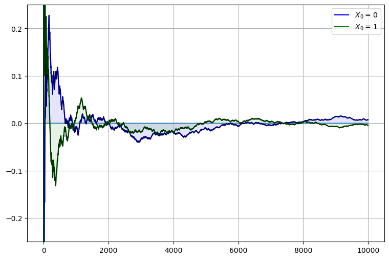
Solution to Exercise 24.1

We will address this exercise graphically.

The plots show the time series of \(\bar X_m - p\) for two initial conditions.

As \(m\) gets large, both series converge to zero.

α = β = 0.1
N = 10000
p = β / (α + β)

P = ((1 - α,       α),               # Careful: P and p are distinct
     (    β,   1 - β))
mc = MarkovChain(P)

fig, ax = plt.subplots(figsize=(9, 6))
ax.set_ylim(-0.25, 0.25)
ax.grid()
ax.hlines(0, 0, N, lw=2, alpha=0.6)   # Horizonal line at zero

for x0, col in ((0, 'blue'), (1, 'green')):
    # Generate time series for worker that starts at x0
    X = mc.simulate(N, init=x0)
    # Compute fraction of time spent unemployed, for each n
    X_bar = (X == 0).cumsum() / (1 + np.arange(N, dtype=float))
    # Plot
    ax.fill_between(range(N), np.zeros(N), X_bar - p, color=col, alpha=0.1)
    ax.plot(X_bar - p, color=col, label=f'$X_0 = \, {x0} $')
    # Overlay in black--make lines clearer
    ax.plot(X_bar - p, 'k-', alpha=0.6)

ax.legend(loc='upper right')
plt.show()

_images/bd31b1102150725f2483b6ced4a060ec964aa356c73c5a7cdae139a5f9fd964a.png

Exercise 24.2

A topic of interest for economics and many other disciplines is ranking.

Let’s now consider one of the most practical and important ranking problems — the rank assigned to web pages by search engines.

(Although the problem is motivated from outside of economics, there is in fact a deep connection between search ranking systems and prices in certain competitive equilibria — see [Du et al., 2013].)

To understand the issue, consider the set of results returned by a query to a web search engine.

For the user, it is desirable to

receive a large set of accurate matches
have the matches returned in order, where the order corresponds to some measure of “importance”

Ranking according to a measure of importance is the problem we now consider.

The methodology developed to solve this problem by Google founders Larry Page and Sergey Brin is known as PageRank.

To illustrate the idea, consider the following diagram

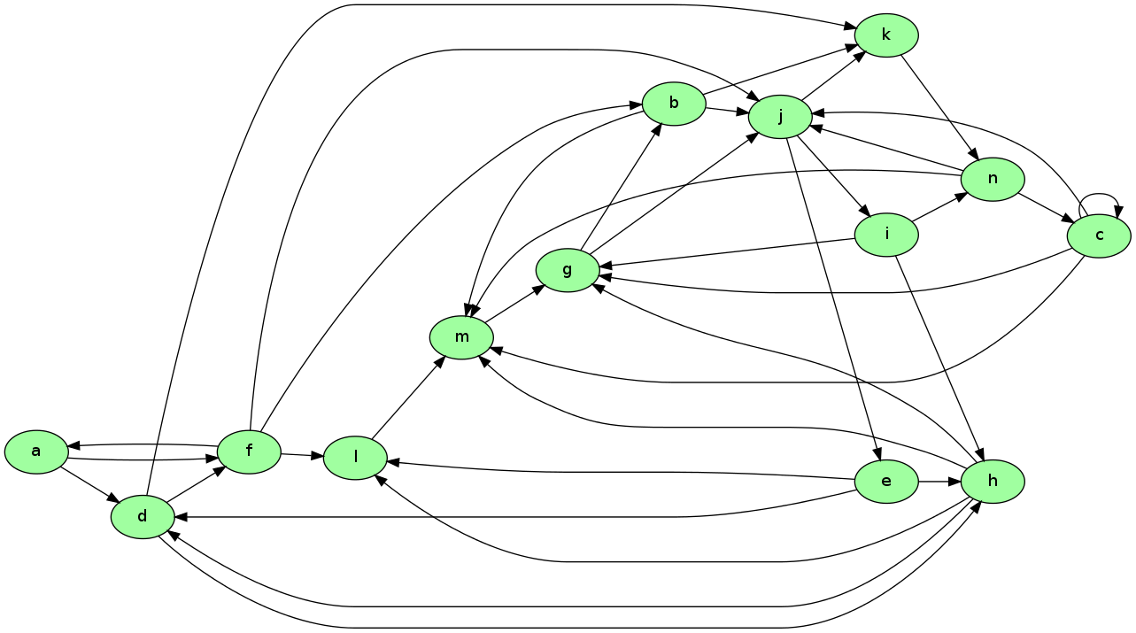
Imagine that this is a miniature version of the WWW, with

each node representing a web page
each arrow representing the existence of a link from one page to another

Now let’s think about which pages are likely to be important, in the sense of being valuable to a search engine user.

One possible criterion for the importance of a page is the number of inbound links — an indication of popularity.

By this measure, m and j are the most important pages, with 5 inbound links each.

However, what if the pages linking to m, say, are not themselves important?

Thinking this way, it seems appropriate to weight the inbound nodes by relative importance.

The PageRank algorithm does precisely this.

A slightly simplified presentation that captures the basic idea is as follows.

Letting \(j\) be (the integer index of) a typical page and \(r_j\) be its ranking, we set

\[ r_j = \sum_{i \in L_j} \frac{r_i}{\ell_i} \]

where

\(\ell_i\) is the total number of outbound links from \(i\)
\(L_j\) is the set of all pages \(i\) such that \(i\) has a link to \(j\)

This is a measure of the number of inbound links, weighted by their own ranking (and normalized by \(1 / \ell_i\)).

There is, however, another interpretation, and it brings us back to Markov chains.

Let \(P\) be the matrix given by \(P(i, j) = \mathbf 1\{i \to j\} / \ell_i\) where \(\mathbf 1\{i \to j\} = 1\) if \(i\) has a link to \(j\) and zero otherwise.

The matrix \(P\) is a stochastic matrix provided that each page has at least one link.

With this definition of \(P\) we have

\[ r_j = \sum_{i \in L_j} \frac{r_i}{\ell_i} = \sum_{\text{all } i} \mathbf 1\{i \to j\} \frac{r_i}{\ell_i} = \sum_{\text{all } i} P(i, j) r_i \]

Writing \(r\) for the row vector of rankings, this becomes \(r = r P\).

Hence \(r\) is the stationary distribution of the stochastic matrix \(P\).

Let’s think of \(P(i, j)\) as the probability of “moving” from page \(i\) to page \(j\).

The value \(P(i, j)\) has the interpretation

\(P(i, j) = 1/k\) if \(i\) has \(k\) outbound links and \(j\) is one of them
\(P(i, j) = 0\) if \(i\) has no direct link to \(j\)

Thus, motion from page to page is that of a web surfer who moves from one page to another by randomly clicking on one of the links on that page.

Here “random” means that each link is selected with equal probability.

Since \(r\) is the stationary distribution of \(P\), assuming that the uniform ergodicity condition is valid, we can interpret \(r_j\) as the fraction of time that a (very persistent) random surfer spends at page \(j\).

Your exercise is to apply this ranking algorithm to the graph pictured above and return the list of pages ordered by rank.

There is a total of 14 nodes (i.e., web pages), the first named a and the last named n.

A typical line from the file has the form

d -> h;

This should be interpreted as meaning that there exists a link from d to h.

The data for this graph is shown below, and read into a file called web_graph_data.txt when the cell is executed.

%%file web_graph_data.txt
a -> d;
a -> f;
b -> j;
b -> k;
b -> m;
c -> c;
c -> g;
c -> j;
c -> m;
d -> f;
d -> h;
d -> k;
e -> d;
e -> h;
e -> l;
f -> a;
f -> b;
f -> j;
f -> l;
g -> b;
g -> j;
h -> d;
h -> g;
h -> l;
h -> m;
i -> g;
i -> h;
i -> n;
j -> e;
j -> i;
j -> k;
k -> n;
l -> m;
m -> g;
n -> c;
n -> j;
n -> m;

Overwriting web_graph_data.txt

To parse this file and extract the relevant information, you can use regular expressions.

The following code snippet provides a hint as to how you can go about this

import re
re.findall('\w', 'x +++ y ****** z')  # \w matches alphanumerics

['x', 'y', 'z']

re.findall('\w', 'a ^^ b &&& $$ c')

['a', 'b', 'c']

When you solve for the ranking, you will find that the highest ranked node is in fact g, while the lowest is a.

Solution to Exercise 24.2

Here is one solution:

"""
Return list of pages, ordered by rank
"""
import re
from operator import itemgetter

infile = 'web_graph_data.txt'
alphabet = 'abcdefghijklmnopqrstuvwxyz'

n = 14 # Total number of web pages (nodes)

# Create a matrix Q indicating existence of links
#  * Q[i, j] = 1 if there is a link from i to j
#  * Q[i, j] = 0 otherwise
Q = np.zeros((n, n), dtype=int)
with open(infile) as f:
    edges = f.readlines()
for edge in edges:
    from_node, to_node = re.findall('\w', edge)
    i, j = alphabet.index(from_node), alphabet.index(to_node)
    Q[i, j] = 1
# Create the corresponding Markov matrix P
P = np.empty((n, n))
for i in range(n):
    P[i, :] = Q[i, :] / Q[i, :].sum()
mc = MarkovChain(P)
# Compute the stationary distribution r
r = mc.stationary_distributions[0]
ranked_pages = {alphabet[i] : r[i] for i in range(n)}
# Print solution, sorted from highest to lowest rank
print('Rankings\n ***')
for name, rank in sorted(ranked_pages.items(), key=itemgetter(1), reverse=1):
    print(f'{name}: {rank:.4}')

Rankings
 ***
g: 0.1607
j: 0.1594
m: 0.1195
n: 0.1088
k: 0.09106
b: 0.08326
e: 0.05312
i: 0.05312
c: 0.04834
h: 0.0456
l: 0.03202
d: 0.03056
f: 0.01164
a: 0.002911

Exercise 24.3

In numerical work, it is sometimes convenient to replace a continuous model with a discrete one.

In particular, Markov chains are routinely generated as discrete approximations to AR(1) processes of the form

\[ y_{t+1} = \rho y_t + u_{t+1} \]

Here \({u_t}\) is assumed to be IID and \(N(0, \sigma_u^2)\).

The variance of the stationary probability distribution of \(\{ y_t \}\) is

\[ \sigma_y^2 := \frac{\sigma_u^2}{1-\rho^2} \]

Tauchen’s method [Tauchen, 1986] is the most common method for approximating this continuous state process with a finite state Markov chain.

A routine for this already exists in QuantEcon.py but let’s write our own version as an exercise.

As a first step, we choose

\(n\), the number of states for the discrete approximation
\(m\), an integer that parameterizes the width of the state space

Next, we create a state space \(\{x_0, \ldots, x_{n-1}\} \subset \mathbb R\) and a stochastic \(n \times n\) matrix \(P\) such that

\(x_0 = - m \, \sigma_y\)
\(x_{n-1} = m \, \sigma_y\)
\(x_{i+1} = x_i + s\) where \(s = (x_{n-1} - x_0) / (n - 1)\)

Let \(F\) be the cumulative distribution function of the normal distribution \(N(0, \sigma_u^2)\).

The values \(P(x_i, x_j)\) are computed to approximate the AR(1) process — omitting the derivation, the rules are as follows:

If \(j = 0\), then set

\[ P(x_i, x_j) = P(x_i, x_0) = F(x_0-\rho x_i + s/2) \]
If \(j = n-1\), then set

\[ P(x_i, x_j) = P(x_i, x_{n-1}) = 1 - F(x_{n-1} - \rho x_i - s/2) \]
Otherwise, set

\[ P(x_i, x_j) = F(x_j - \rho x_i + s/2) - F(x_j - \rho x_i - s/2) \]

The exercise is to write a function approx_markov(rho, sigma_u, m=3, n=7) that returns \(\{x_0, \ldots, x_{n-1}\} \subset \mathbb R\) and \(n \times n\) matrix \(P\) as described above.

Even better, write a function that returns an instance of QuantEcon.py’s MarkovChain class.

Solution to Exercise 24.3

A solution from the QuantEcon.py library can be found here.

1: Hint: First show that if \(P\) and \(Q\) are stochastic matrices then so is their product — to check the row sums, try post multiplying by a column vector of ones. Finally, argue that \(P^n\) is a stochastic matrix using induction.