8. Elementary Probability with Matrices#
This lecture uses matrix algebra to illustrate some basic ideas about probability theory.
After introducing underlying objects, we’ll use matrices and vectors to describe probability distributions.
Among concepts that we’ll be studying include
a joint probability distribution
marginal distributions associated with a given joint distribution
conditional probability distributions
statistical independence of two random variables
joint distributions associated with a prescribed set of marginal distributions
couplings
copulas
the probability distribution of a sum of two independent random variables
convolution of marginal distributions
parameters that define a probability distribution
sufficient statistics as data summaries
We’ll use a matrix to represent a bivariate or multivariate probability distribution and a vector to represent a univariate probability distribution
This companion lecture describes some popular probability distributions and describes how to use Python to sample from them.
In addition to what’s in Anaconda, this lecture will need the following libraries:
!pip install prettytable
As usual, we’ll start with some imports
import numpy as np
import matplotlib.pyplot as plt
import prettytable as pt
from scipy import stats
from scipy.special import comb
from mpl_toolkits.mplot3d import Axes3D
from matplotlib_inline.backend_inline import set_matplotlib_formats
set_matplotlib_formats('retina')

rng = np.random.default_rng(0)
8.1. Sketch of basic concepts#
We’ll briefly define what we mean by a probability space, a probability measure, and a random variable.
For most of this lecture, we sweep these objects into the background
Note
Nevertheless, they’ll be lurking beneath induced distributions of random variables that we’ll focus on here.
These deeper objects are essential for defining and analysing the concepts of stationarity and ergodicity that underly laws of large numbers.
For a relatively nontechnical presentation of some of these results see this chapter from Lars Peter Hansen and Thomas J. Sargent’s online monograph titled Risk, Uncertainty, and Values.
Let \(\Omega\) be a set of possible underlying outcomes and let \(\omega \in \Omega\) be a particular underlying outcome.
Let \(\mathcal{F}\) be a collection of subsets of \(\Omega\) that we call events.
(Technically, \(\mathcal{F}\) is a \(\sigma\)-algebra.)
A probability measure \(\mu\) maps each event \(\mathcal{G} \in \mathcal{F}\) into a scalar number \(\mu(\mathcal{G})\) between \(0\) and \(1\), with \(\mu(\Omega)=1\).
The triple \(\Omega,\mathcal{F},\mu\) forms our probability space.
A random variable \(X(\omega)\) is a function of the underlying outcome \(\omega \in \Omega\) that assigns a value in some set of possible values.
If \(A\) is a set of possible values of \(X\), then the event that \(X\) lies in \(A\) is
The random variable \(X(\omega)\) has a probability distribution induced by the probability measure \(\mu\):
If \(\mu\) has a density \(p(\omega)\), then we can also write
We call this the induced probability distribution of random variable \(X\).
Instead of working explicitly with an underlying probability space \(\Omega,\mathcal{F}\) and probability measure \(\mu\), applied statisticians often proceed simply by specifying a form for an induced distribution for a random variable \(X\).
That is how we’ll proceed in this lecture and in many subsequent lectures.
8.2. What does probability mean?#
Before diving in, we’ll say a few words about what probability theory means and how it connects to statistics.
We also touch on these topics in Two Meanings of Probability and Bayesian versus Frequentist Decision Rules.
For much of this lecture we’ll be discussing fixed “population” probabilities.
These are purely mathematical objects.
To appreciate how statisticians connect probabilities to data, the key is to understand the following concepts:
A single draw from a probability distribution
Repeated independently and identically distributed (i.i.d.) draws of “samples” or “realizations” from the same probability distribution
A statistic defined as a function of a sequence of samples
An empirical distribution or histogram (a binned empirical distribution) that records observed relative frequencies
The idea that a population probability distribution is what we anticipate relative frequencies will be in a long sequence of i.i.d. draws. Here the following mathematical machinery makes precise what is meant by anticipated relative frequencies
Law of Large Numbers (LLN)
Central Limit Theorem (CLT)
8.2.1. A discrete random variable example#
8.2.1.1. Scalar example#
Let \(X\) be a scalar random variable that takes on the \(I\) possible values \(0, 1, 2, \ldots, I-1\) with probabilities
where
We sometimes write
as a short-hand way of saying that the random variable \(X\) is described by the probability distribution \( \{{f_i}\}_{i=0}^{I-1}\).
Consider drawing a sample \(x_0, x_1, \dots , x_{N-1}\) of \(N\) independent and identically distributed draws of \(X\).
What do “identical” and “independent” mean in IID or iid (“identically and independently distributed”)?
“identical” means that each draw is from the same distribution.
“independent” means that the joint distribution equals the product of marginal distributions, i.e.,
We define an empirical distribution as follows.
For each \(i = 0,\dots,I-1\), let
Key concepts that connect probability theory with statistics are laws of large numbers and central limit theorems.
A Law of Large Numbers (LLN) states that \(\tilde {f_i} \to f_i\) as \(N \to \infty\).
A Central Limit Theorem (CLT) describes a rate at which \(\tilde {f_i} \to f_i\).
See LLN and CLT for a detailed treatment of both results.
8.2.2. Understanding probability: frequentist vs. Bayesian#
For “frequentist” statisticians, anticipated relative frequency is all that a probability distribution means.
But for a Bayesian it means something else – something partly subjective and purely personal.
We say “partly” because a Bayesian also pays attention to relative frequencies.
8.3. Representing probability distributions#
A probability distribution \(\textrm{Prob} (X \in A)\) can be described by its cumulative distribution function (CDF)
Sometimes, but not always, a random variable can also be described by a density function \(f(x)\) that is related to its CDF by
Here \(B\) is a set of possible \(X\)’s whose probability of occurring we want to compute.
When a probability density exists, a probability distribution can be characterized either by its CDF or by its density.
For a discrete-valued random variable
the number of possible values of \(X\) is finite or countably infinite
we replace a density with a probability mass function, a non-negative sequence that sums to one
when a density exists, we replace integration with summation in formulas like (8.1)
In this lecture, we mostly discuss discrete random variables.
Doing this enables us to confine our tool set basically to linear algebra.
Later we’ll briefly discuss how to approximate a continuous random variable with a discrete random variable.
8.4. Univariate probability distributions#
We’ll devote most of this lecture to discrete-valued random variables, but we’ll say a few things about continuous-valued random variables.
8.4.1. Discrete random variable#
Let \(X\) be a discrete random variable that takes possible values: \(i=0,1,\ldots,I-1 = \bar{X}\).
Here, we choose the maximum index \(I-1\) because of how this aligns nicely with Python’s index convention.
Define \(f_i \equiv \textrm{Prob}\{X=i\}\) and assemble the non-negative vector
for which \(f_{i} \in [0,1]\) for each \(i\) and \(\sum_{i=0}^{I-1}f_i=1\).
This vector defines a probability mass function.
The distribution (8.2) has parameters \(\{f_{i}\}_{i=0,1, \cdots ,I-2}\) since \(f_{I-1} = 1-\sum_{i=0}^{I-2}f_{i}\).
These parameters pin down the shape of the distribution.
(Sometimes \(I = \infty\).)
Such a “non-parametric” distribution has as many “parameters” as there are possible values of the random variable.
We often work with special distributions that are characterized by a small number parameters.
In these special parametric distributions,
where \(\theta \) is a vector of parameters that is of much smaller dimension than \(I\).
A statistical model is a joint probability distribution characterized by a list of parameters.
The concept of parameter is intimately related to the notion of sufficient statistic.
A statistic is a nonlinear function of a data set.
Sufficient statistics summarize all information that a data set contains about parameters of a statistical model.
Note that a sufficient statistic corresponds to a particular statistical model.
Sufficient statistics are key tools that AI uses to summarize or compress a big data set.
R. A. Fisher provided a rigorous definition of information – see Fisher information.
An example of a parametric probability distribution is a geometric distribution.
It is described by
Evidently, \(\sum_{i=0}^{\infty}f_i=1\).
Let \(\theta\) be a vector of parameters of the distribution described by \(f\), then
8.4.2. Continuous random variable#
Let \(X\) be a continuous random variable that takes values in a set \(\tilde{X} \subseteq \mathbb{R}\) and whose distribution has parameters \(\theta\).
where \(A\) is a subset of \(\tilde{X}\) and
8.5. Bivariate probability distributions#
We’ll now discuss a bivariate joint distribution.
To begin, we restrict ourselves to two discrete random variables.
Let \(X,Y\) be two discrete random variables that take values:
Then their joint distribution is described by a matrix
whose elements are
where
8.6. Marginal probability distributions#
The joint distribution induces marginal distributions
For example, let a joint distribution over \((X,Y)\) be
The implied marginal distributions are:
As a digression, if two random variables \(X,Y\) are continuous and have joint density \(f(x,y)\), then marginal distributions can be computed by
8.7. Conditional probability distributions#
Conditional probabilities are defined according to
where \(A, B\) are two events.
For a pair of discrete random variables, we have the conditional distribution
where \(i=0, \ldots,I-1, \quad j=0,\ldots,J-1\).
Note that
The mathematics of conditional probability implies:
Note
Formula (8.4) is also what a Bayesian calls Bayes’ Law.
A Bayesian statistician regards marginal probability distribution \(\textrm{Prob}({X=i}), i = 0, \ldots, I-1\) as a prior distribution that describes his personal subjective beliefs about \(X\).
He then interprets formula (8.4) as a procedure for constructing a posterior distribution that describes how he would revise his subjective beliefs after observing that \(Y\) equals \(j\).
For the joint distribution (8.3)
8.8. Transition probability matrix#
Consider the following joint probability distribution of two random variables.
Let \(X,Y\) be discrete random variables with joint distribution
where \(i = 0,\dots,I-1; j = 0,\dots,J-1\) and
An associated conditional distribution is
We can define a transition probability matrix \(P\) with \(i,j\) component
where
The first row is the probability that \(Y=j, j=0,1\) conditional on \(X=0\).
The second row is the probability that \(Y=j, j=0,1\) conditional on \(X=1\).
Note that
\(\sum_{j}p_{ij}= \frac{ \sum_{j}\rho_{ij}}{ \sum_{j}\rho_{ij}}=1\), so each row of the transition matrix \(P\) is a probability distribution (not so for each column).
8.9. Application: forecasting a time series#
Suppose that there are two time periods.
\(t=0\) “today”
\(t=1\) “tomorrow”
Let \(X(0)\) be a random variable to be realized at \(t=0\), \(X(1)\) be a random variable to be realized at \(t=1\).
Suppose that
\(f_{ij} \) is a joint distribution over \([X(0), X(1)]\).
A conditional distribution is
This formula is a workhorse for applied economic forecasters.
8.10. Statistical independence#
Random variables X and Y are statistically independent if
where
Conditional distributions are
8.11. Means and variances#
The mean and variance of a discrete random variable \(X\) are
A continuous random variable having density \(f_{X}(x)\) has mean and variance
8.12. Matrix representations of some bivariate distributions#
Let’s use matrices to represent a joint distribution, conditional distribution, marginal distribution, and the mean and variance of a bivariate random variable.
The table below illustrates a probability distribution for a bivariate random variable.
Marginal distributions are
Let’s write some Python code that lets us draw some long samples and compute relative frequencies.
The code lets us check whether the “sampling” distribution agrees with the “population” distribution – confirming that the population distribution correctly tells us the relative frequencies that we should expect in a large sample.
# specify parameters
xs = np.array([0, 1])
ys = np.array([10, 20])
f = np.array([[0.3, 0.2], [0.1, 0.4]])
f_cum = np.cumsum(f)

# draw random numbers
p = rng.random(1_000_000)
x = np.vstack([xs[1]*np.ones(p.shape), ys[1]*np.ones(p.shape)])
# map to the bivariate distribution

x[0, p < f_cum[2]] = xs[1]
x[1, p < f_cum[2]] = ys[0]

x[0, p < f_cum[1]] = xs[0]
x[1, p < f_cum[1]] = ys[1]

x[0, p < f_cum[0]] = xs[0]
x[1, p < f_cum[0]] = ys[0]
print(x)
[[ 1.  0.  0. ...  0.  0.  0.]
 [20. 10. 10. ... 10. 10. 20.]]
Note
To generate random draws from the joint distribution \(F\), we use the inverse CDF technique described in this companion lecture.
# marginal distribution
xp = np.sum(x[0, :] == xs[0])/1_000_000
yp = np.sum(x[1, :] == ys[0])/1_000_000

# print output
print("marginal distribution for x")
xmtb = pt.PrettyTable()
xmtb.field_names = ['x_value', 'x_prob']
xmtb.add_row([xs[0], xp])
xmtb.add_row([xs[1], 1-xp])
print(xmtb)

print("\nmarginal distribution for y")
ymtb = pt.PrettyTable()
ymtb.field_names = ['y_value', 'y_prob']
ymtb.add_row([ys[0], yp])
ymtb.add_row([ys[1], 1-yp])
print(ymtb)
marginal distribution for x
+---------+----------+
| x_value |  x_prob  |
+---------+----------+
|    0    | 0.500194 |
|    1    | 0.499806 |
+---------+----------+

marginal distribution for y
+---------+----------+
| y_value |  y_prob  |
+---------+----------+
|    10   | 0.399741 |
|    20   | 0.600259 |
+---------+----------+
# conditional distributions
xc1 = x[0, x[1, :] == ys[0]]
xc2 = x[0, x[1, :] == ys[1]]
yc1 = x[1, x[0, :] == xs[0]]
yc2 = x[1, x[0, :] == xs[1]]

xc1p = np.sum(xc1 == xs[0])/len(xc1)
xc2p = np.sum(xc2 == xs[0])/len(xc2)
yc1p = np.sum(yc1 == ys[0])/len(yc1)
yc2p = np.sum(yc2 == ys[0])/len(yc2)

# print output
print("conditional distribution for x")
xctb = pt.PrettyTable()
xctb.field_names = ['y_value', 'prob(x=0)', 'prob(x=1)']
xctb.add_row([ys[0], xc1p, 1-xc1p])
xctb.add_row([ys[1], xc2p, 1-xc2p])
print(xctb)

print("\nconditional distribution for y")
yctb = pt.PrettyTable()
yctb.field_names = ['x_value',  'prob(y=10)', 'prob(y=20)']
yctb.add_row([xs[0], yc1p, 1-yc1p])
yctb.add_row([xs[1], yc2p, 1-yc2p])
print(yctb)
conditional distribution for x
+---------+--------------------+---------------------+
| y_value |     prob(x=0)      |      prob(x=1)      |
+---------+--------------------+---------------------+
|    10   | 0.7504634250677313 | 0.24953657493226866 |
|    20   | 0.333527693878809  |  0.666472306121191  |
+---------+--------------------+---------------------+

conditional distribution for y
+---------+---------------------+---------------------+
| x_value |      prob(y=10)     |      prob(y=20)     |
+---------+---------------------+---------------------+
|    0    |  0.5997492972726582 | 0.40025070272734176 |
|    1    | 0.19957743604518552 |  0.8004225639548145 |
+---------+---------------------+---------------------+
Let’s calculate population marginal and conditional probabilities using matrix algebra.
\(\implies\)
(1) Marginal distribution:
(2) Conditional distribution:
These population objects closely resemble the sample counterparts computed above.
Let’s wrap some of the functions we have used in a Python class that will let us generate and sample from a discrete bivariate joint distribution.
class discrete_bijoint:

    def __init__(self, f, xs, ys):
        '''initialization
        -----------------
        parameters:
        f: the bivariate joint probability matrix
        xs: values of x vector
        ys: values of y vector
        '''
        self.f, self.xs, self.ys = f, xs, ys

    def joint_tb(self):
        '''print the joint distribution table'''
        xs = self.xs
        ys = self.ys
        f = self.f
        jtb = pt.PrettyTable()
        jtb.field_names = ['x_value/y_value', *ys, 'marginal sum for x']
        for i in range(len(xs)):
            jtb.add_row([xs[i], *f[i, :], np.sum(f[i, :])])
        jtb.add_row(['marginal_sum for y', *np.sum(f, 0), np.sum(f)])
        print("\nThe joint probability distribution for x and y\n", jtb)
        self.jtb = jtb

    def draw(self, n):
        '''draw random numbers
        ----------------------
        parameters:
        n: number of random numbers to draw
        '''
        xs = self.xs
        ys = self.ys
        f_cum = np.cumsum(self.f)
        p = rng.random(n)
        x = np.empty([2, p.shape[0]])
        lf = len(f_cum)
        lx = len(xs)-1
        ly = len(ys)-1
        for i in range(lf):
            x[0, p < f_cum[lf-1-i]] = xs[lx]
            x[1, p < f_cum[lf-1-i]] = ys[ly]
            if ly == 0:
                lx -= 1
                ly = len(ys)-1
            else:
                ly -= 1
        self.x = x
        self.n = n

    def marg_dist(self):
        '''marginal distribution'''
        x = self.x
        xs = self.xs
        ys = self.ys
        n = self.n
        xmp = [np.sum(x[0, :] == xs[i])/n for i in range(len(xs))]
        ymp = [np.sum(x[1, :] == ys[i])/n for i in range(len(ys))]

        # print output
        xmtb = pt.PrettyTable()
        ymtb = pt.PrettyTable()
        xmtb.field_names = ['x_value', 'x_prob']
        ymtb.field_names = ['y_value', 'y_prob']
        for i in range(max(len(xs), len(ys))):
            if i < len(xs):
                xmtb.add_row([xs[i], xmp[i]])
            if i < len(ys):
                ymtb.add_row([ys[i], ymp[i]])
        xmtb.add_row(['sum', np.sum(xmp)])
        ymtb.add_row(['sum', np.sum(ymp)])
        print("\nmarginal distribution for x\n", xmtb)
        print("\nmarginal distribution for y\n", ymtb)

        self.xmp = xmp
        self.ymp = ymp

    def cond_dist(self):
        '''conditional distribution'''
        x = self.x
        xs = self.xs
        ys = self.ys
        n = self.n
        xcp = np.empty([len(ys), len(xs)])
        ycp = np.empty([len(xs), len(ys)])
        for i in range(max(len(ys), len(xs))):
            if i < len(ys):
                xi = x[0, x[1, :] == ys[i]]
                idx = xi.reshape(len(xi), 1) == xs.reshape(1, len(xs))
                xcp[i, :] = np.sum(idx, 0)/len(xi)
            if i < len(xs):
                yi = x[1, x[0, :] == xs[i]]
                idy = yi.reshape(len(yi), 1) == ys.reshape(1, len(ys))
                ycp[i, :] = np.sum(idy, 0)/len(yi)

        # print output
        xctb = pt.PrettyTable()
        yctb = pt.PrettyTable()
        xctb.field_names = ['x_value', *xs, 'sum']
        yctb.field_names = ['y_value', *ys, 'sum']
        for i in range(max(len(xs), len(ys))):
            if i < len(ys):
                xctb.add_row([ys[i], *xcp[i], np.sum(xcp[i])])
            if i < len(xs):
                yctb.add_row([xs[i], *ycp[i], np.sum(ycp[i])])
        print("\nconditional distribution for x\n", xctb)
        print("\nconditional distribution for y\n", yctb)

        self.xcp = xcp
        self.xyp = ycp
Let’s apply our code to some examples.
8.12.1. Numerical examples#
8.12.1.1. Example 1#
# joint
d = discrete_bijoint(f, xs, ys)
d.joint_tb()
The joint probability distribution for x and y
 +--------------------+-----+--------------------+--------------------+
|  x_value/y_value   |  10 |         20         | marginal sum for x |
+--------------------+-----+--------------------+--------------------+
|         0          | 0.3 |        0.2         |        0.5         |
|         1          | 0.1 |        0.4         |        0.5         |
| marginal_sum for y | 0.4 | 0.6000000000000001 |        1.0         |
+--------------------+-----+--------------------+--------------------+
# sample marginal
d.draw(1_000_000)
d.marg_dist()
marginal distribution for x
 +---------+----------+
| x_value |  x_prob  |
+---------+----------+
|    0    | 0.499395 |
|    1    | 0.500605 |
|   sum   |   1.0    |
+---------+----------+

marginal distribution for y
 +---------+----------+
| y_value |  y_prob  |
+---------+----------+
|    10   | 0.400501 |
|    20   | 0.599499 |
|   sum   |   1.0    |
+---------+----------+
# sample conditional
d.cond_dist()
conditional distribution for x
 +---------+--------------------+---------------------+-----+
| x_value |         0          |          1          | sum |
+---------+--------------------+---------------------+-----+
|    10   | 0.7491766562380618 | 0.25082334376193816 | 1.0 |
|    20   | 0.3325259925371018 |  0.6674740074628982 | 1.0 |
+---------+--------------------+---------------------+-----+

conditional distribution for y
 +---------+---------------------+--------------------+-----+
| y_value |          10         |         20         | sum |
+---------+---------------------+--------------------+-----+
|    0    |  0.6008189909790846 | 0.3991810090209153 | 1.0 |
|    1    | 0.20066719269683683 | 0.7993328073031631 | 1.0 |
+---------+---------------------+--------------------+-----+
8.12.1.2. Example 2#
xs_new = np.array([10, 20, 30])
ys_new = np.array([1, 2])
f_new = np.array([[0.2, 0.1], [0.1, 0.3], [0.15, 0.15]])
d_new = discrete_bijoint(f_new, xs_new, ys_new)
d_new.joint_tb()
The joint probability distribution for x and y
 +--------------------+---------------------+------+---------------------+
|  x_value/y_value   |          1          |  2   |  marginal sum for x |
+--------------------+---------------------+------+---------------------+
|         10         |         0.2         | 0.1  | 0.30000000000000004 |
|         20         |         0.1         | 0.3  |         0.4         |
|         30         |         0.15        | 0.15 |         0.3         |
| marginal_sum for y | 0.45000000000000007 | 0.55 |         1.0         |
+--------------------+---------------------+------+---------------------+
d_new.draw(1_000_000)
d_new.marg_dist()
marginal distribution for x
 +---------+----------+
| x_value |  x_prob  |
+---------+----------+
|    10   | 0.299848 |
|    20   | 0.401015 |
|    30   | 0.299137 |
|   sum   |   1.0    |
+---------+----------+

marginal distribution for y
 +---------+----------+
| y_value |  y_prob  |
+---------+----------+
|    1    | 0.449195 |
|    2    | 0.550805 |
|   sum   |   1.0    |
+---------+----------+
d_new.cond_dist()
conditional distribution for x
 +---------+---------------------+---------------------+--------------------+-----+
| x_value |          10         |          20         |         30         | sum |
+---------+---------------------+---------------------+--------------------+-----+
|    1    |  0.4445886530348735 | 0.22256258417836353 | 0.332848762786763  | 1.0 |
|    2    | 0.18180844400468404 |  0.5465473261862184 | 0.2716442298090976 | 1.0 |
+---------+---------------------+---------------------+--------------------+-----+

conditional distribution for y
 +---------+---------------------+--------------------+-----+
| y_value |          1          |         2          | sum |
+---------+---------------------+--------------------+-----+
|    10   |  0.6660274539099811 | 0.3339725460900189 | 1.0 |
|    20   | 0.24930239517225042 | 0.7506976048277496 | 1.0 |
|    30   |  0.4998178092312218 | 0.5001821907687782 | 1.0 |
+---------+---------------------+--------------------+-----+
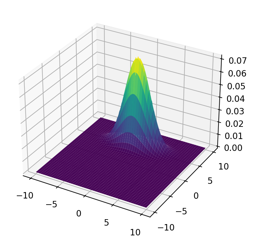
8.13. A continuous bivariate random vector#
A two-dimensional Gaussian distribution has joint density
We start with a bivariate normal distribution pinned down by
# define the joint probability density function
def func(x, y, μ1=0, μ2=5, σ1=np.sqrt(5), σ2=np.sqrt(1), ρ=.2/np.sqrt(5*1)):
    A = (2 * np.pi * σ1 * σ2 * np.sqrt(1 - ρ**2))**(-1)
    B = -1 / 2 / (1 - ρ**2)
    C1 = (x - μ1)**2 / σ1**2
    C2 = 2 * ρ * (x - μ1) * (y - μ2) / σ1 / σ2
    C3 = (y - μ2)**2 / σ2**2
    return A * np.exp(B * (C1 - C2 + C3))
μ1 = 0
μ2 = 5
σ1 = np.sqrt(5)
σ2 = np.sqrt(1)
ρ = .2 / np.sqrt(5 * 1)
x = np.linspace(-10, 10, 1_000)
y = np.linspace(-10, 10, 1_000)
x_mesh, y_mesh = np.meshgrid(x, y, indexing="ij")
8.13.1. Joint, marginal, and conditional distributions#
8.13.1.1. Joint distribution#
Let’s plot the population joint density.
# %matplotlib notebook

fig = plt.figure()
ax = plt.axes(projection='3d')

surf = ax.plot_surface(x_mesh, y_mesh, func(x_mesh, y_mesh), cmap='viridis')
plt.show()
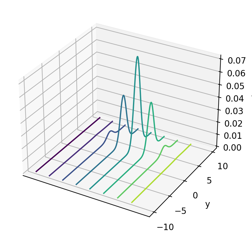
# %matplotlib notebook

fig = plt.figure()
ax = plt.axes(projection='3d')

curve = ax.contour(x_mesh, y_mesh, func(x_mesh, y_mesh), zdir='x')
plt.ylabel('y')
ax.set_zlabel('f')
ax.set_xticks([])
plt.show()
Next we can use a built-in numpy function to draw random samples, then calculate a sample marginal distribution from the sample mean and variance.
μ= np.array([0, 5])
σ= np.array([[5, .2], [.2, 1]])
n = 1_000_000
data = rng.multivariate_normal(μ, σ, n)
x = data[:, 0]
y = data[:, 1]
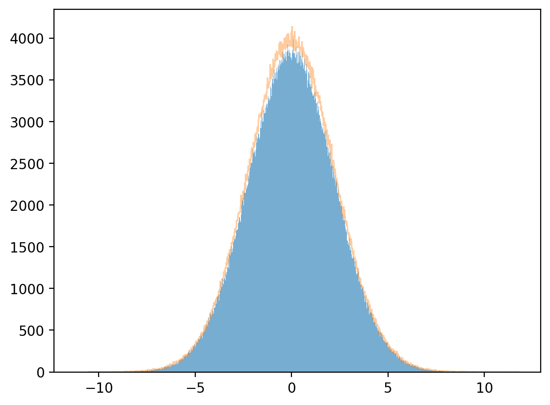
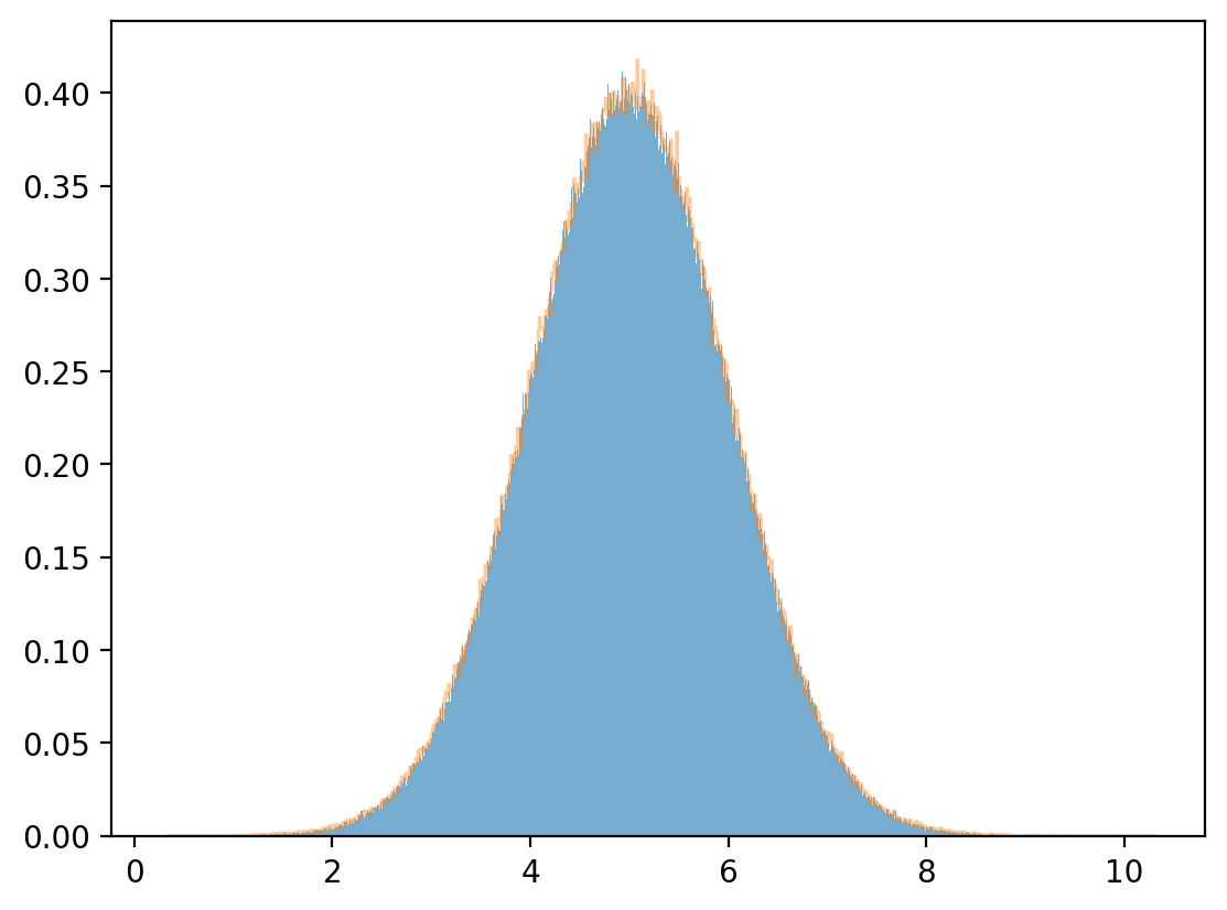
8.13.1.2. Marginal distribution#
plt.hist(x, bins=1_000, alpha=0.6)
μx_hat, σx_hat = np.mean(x), np.std(x)
print(μx_hat, σx_hat)
x_sim = rng.normal(μx_hat, σx_hat, 1_000_000)
plt.hist(x_sim, bins=1_000, alpha=0.4, histtype="step")
plt.show()
-0.002835018476282638 2.237281153907461
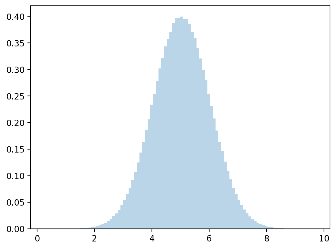
plt.hist(y, bins=1_000, density=True, alpha=0.6)
μy_hat, σy_hat = np.mean(y), np.std(y)
print(μy_hat, σy_hat)
y_sim = rng.normal(μy_hat, σy_hat, 1_000_000)
plt.hist(y_sim, bins=1_000, density=True, alpha=0.4, histtype="step")
plt.show()
4.998242637632656 0.9993565018250069
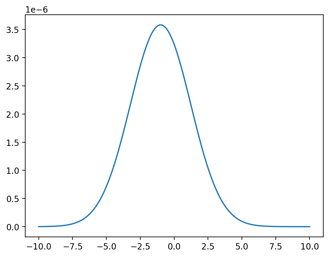
8.13.1.3. Conditional distribution#
For a bivariate normal population distribution, the conditional distributions are also normal:
Note
Please see this quantecon lecture for more details.
Let’s approximate the joint density by discretizing and mapping the approximating joint density into a matrix.
On an evenly spaced grid, we can approximate the conditional distribution by assigning probability weights proportional to a slice of the joint density.
For fixed \(y\), this means that
Fix \(y=0\).
# discretized conditional distribution of X given Y = 0
x = np.linspace(-10, 10, 1_000_000)
z = func(x, y=0) / np.sum(func(x, y=0))
plt.plot(x, z)
plt.show()
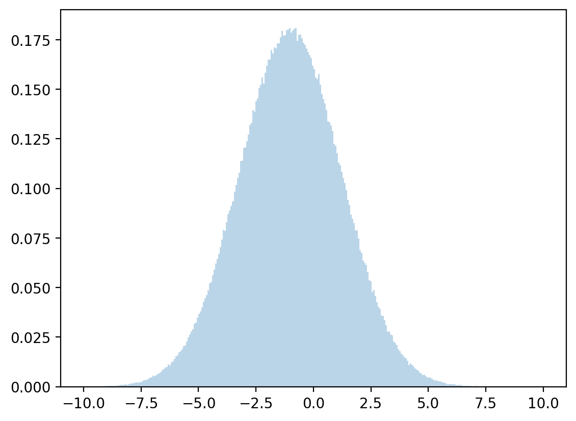
The conditional mean and variance are then approximated by
Let’s draw from a normal distribution with above mean and variance and check how accurate our approximation is.
# discretized mean
μx = np.dot(x, z)

# discretized standard deviation
σx = np.sqrt(np.dot((x - μx)**2, z))

# sample
zz = rng.normal(μx, σx, 1_000_000)
plt.hist(zz, bins=300, density=True, alpha=0.3, range=[-10, 10])
plt.show()
Fix \(x=1\).
y = np.linspace(-10, 10, 1_000_000)
z = func(x=1, y=y) / np.sum(func(x=1, y=y))
plt.plot(y,z)
plt.show()
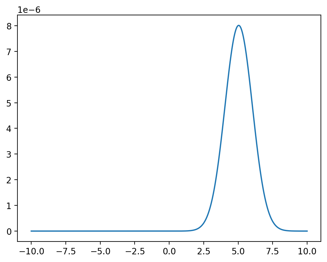
# discretized conditional mean and standard deviation
μy = np.dot(y,z)
σy = np.sqrt(np.dot((y - μy)**2, z))

# sample
zz = rng.normal(μy, σy, 1_000_000)
plt.hist(zz, bins=100, density=True, alpha=0.3)
plt.show()
We compare with the analytically computed parameters and note that they are close.
print(μx, σx)
print(μ1 + ρ * σ1 * (0 - μ2) / σ2, np.sqrt(σ1**2 * (1 - ρ**2)))

print(μy, σy)
print(μ2 + ρ * σ2 * (1 - μ1) / σ1, np.sqrt(σ2**2 * (1 - ρ**2)))
-0.9997518414498444 2.2265841331697698
-1.0 2.227105745132009
5.039998363587647 0.9959878931873033
5.04 0.9959919678390986
8.14. Sum of two independently distributed random variables#
Let \(X, Y\) be two independent discrete random variables that take values in \(\bar{X}, \bar{Y}\), respectively.
Define a new random variable \(Z=X+Y\).
Evidently, \(Z\) takes values from \(\bar{Z}\) defined as follows:
Independence of \(X\) and \( Y\) implies that
Thus, we have:
where \(f * g\) denotes the convolution of the \(f\) and \(g\) sequences.
Similarly, for two random variables \(X,Y\) with densities \(f_{X}, g_{Y}\), the density of \(Z=X+Y\) is
where \( f_{X}*g_{Y} \) denotes the convolution of the \(f_X\) and \(g_Y\) functions.
8.15. Coupling#
Start with a joint distribution
where
From the joint distribution, we have shown above that we obtain unique marginal distributions.
Now we’ll try to go in a reverse direction.
We’ll find that from two marginal distributions we can usually construct more than one joint distribution that satisfies these marginals.
Each of these joint distributions is called a coupling of the two marginal distributions.
Let’s start with marginal distributions
Given two marginal distributions, \(\mu\) for \(X\) and \(\nu\) for \(Y\), a joint distribution \(f_{ij}\) is said to be a coupling of \(\mu\) and \(\nu\).
Consider the following bivariate example.
We construct two couplings.
The first coupling of our two marginal distributions is the joint distribution
To verify that it is a coupling, we check that
A second coupling of our two marginal distributions is the joint distribution
To verify that this is a coupling, note that
Thus, our two proposed joint distributions have the same marginal distributions.
But the joint distributions differ.
Thus, multiple joint distributions \([f_{ij}]\) can have the same marginals.
Couplings are important in optimal transport problems and in Markov processes. Please see this lecture about optimal transport.
8.16. Copula functions#
Suppose that \(X_1, X_2, \dots, X_N\) are \(N\) random variables and that
their marginal distributions are \(F_1(x_1), F_2(x_2),\dots, F_N(x_N)\), and
their joint distribution is \(H(x_1,x_2,\dots,x_N)\)
Then there exists a copula function \(C(\cdot)\) that verifies
If the marginal distributions are continuous, then the copula is unique.
In that case, we can recover it from the marginal inverses:
When marginal distributions are not continuous, one uses generalized inverses, and the copula is uniquely determined only on \(\textrm{Ran}(F_1)\times \cdots \times \textrm{Ran}(F_N)\).
In a reverse direction of logic, given univariate marginal distributions \(F_1(x_1), F_2(x_2),\dots,F_N(x_N)\) and a copula function \(C(\cdot)\), the function \(H(x_1,x_2,\dots,x_N) = C(F_1(x_1), F_2(x_2),\dots,F_N(x_N))\) is a coupling of \(F_1(x_1), F_2(x_2),\dots,F_N(x_N)\).
Thus, for given marginal distributions, we can use a copula function to determine a joint distribution when the associated univariate random variables are not independent.
Copula functions are often used to characterize dependence of random variables.
8.16.1. Bivariate examples with discrete and continuous distributions#
8.16.1.1. Discrete marginal distribution#
As mentioned above, for two given marginal distributions there can be more than one coupling.
For example, consider two random variables \(X, Y\) with distributions
For these two random variables there can be more than one coupling.
Let’s first generate X and Y.
μ = np.array([0.6, 0.4])
ν = np.array([0.3, 0.7])

# number of draws
draws = 1_000_000

# generate independent draws from uniform distribution for X and Y
p_x = rng.random(draws)
p_y = rng.random(draws)

# generate draws of X and Y via independent uniform draws
x = np.ones(draws)
y = np.ones(draws)
x[p_x <= μ[0]] = 0
x[p_x > μ[0]] = 1
y[p_y <= ν[0]] = 0
y[p_y > ν[0]] = 1
# calculate parameters from draws
q_hat = sum(x[x == 1])/draws
r_hat = sum(y[y == 1])/draws

# print output
print("distribution for x")
xmtb = pt.PrettyTable()
xmtb.field_names = ['x_value', 'x_prob']
xmtb.add_row([0, 1-q_hat])
xmtb.add_row([1, q_hat])
print(xmtb)

print("distribution for y")
ymtb = pt.PrettyTable()
ymtb.field_names = ['y_value', 'y_prob']
ymtb.add_row([0, 1-r_hat])
ymtb.add_row([1, r_hat])
print(ymtb)
distribution for x
+---------+----------+
| x_value |  x_prob  |
+---------+----------+
|    0    | 0.599645 |
|    1    | 0.400355 |
+---------+----------+
distribution for y
+---------+---------------------+
| y_value |        y_prob       |
+---------+---------------------+
|    0    | 0.30042599999999997 |
|    1    |       0.699574      |
+---------+---------------------+
Let’s now take our two marginal distributions, one for \(X\), the other for \(Y\), and construct two distinct couplings.
For the first joint distribution:
where
Let’s use Python to construct this joint distribution and then verify that its marginal distributions are what we want.
# define parameters
f1 = np.array([[0.18, 0.42], [0.12, 0.28]])
f1_cum = np.cumsum(f1)

# number of draws
draws1 = 1_000_000

# generate draws from uniform distribution
p = rng.random(draws1)

# generate draws of first coupling via uniform distribution
c1 = np.vstack([np.ones(draws1), np.ones(draws1)])
# X=0, Y=0
c1[0, p <= f1_cum[0]] = 0
c1[1, p <= f1_cum[0]] = 0
# X=0, Y=1
c1[0, (p > f1_cum[0])*(p <= f1_cum[1])] = 0
c1[1, (p > f1_cum[0])*(p <= f1_cum[1])] = 1
# X=1, Y=0
c1[0, (p > f1_cum[1])*(p <= f1_cum[2])] = 1
c1[1, (p > f1_cum[1])*(p <= f1_cum[2])] = 0
# X=1, Y=1
c1[0, (p > f1_cum[2])*(p <= f1_cum[3])] = 1
c1[1, (p > f1_cum[2])*(p <= f1_cum[3])] = 1
# calculate parameters from draws
f1_00 = sum((c1[0, :] == 0)*(c1[1, :] == 0))/draws1
f1_01 = sum((c1[0, :] == 0)*(c1[1, :] == 1))/draws1
f1_10 = sum((c1[0, :] == 1)*(c1[1, :] == 0))/draws1
f1_11 = sum((c1[0, :] == 1)*(c1[1, :] == 1))/draws1

# print output of first joint distribution
print("first joint distribution for c1")
c1_mtb = pt.PrettyTable()
c1_mtb.field_names = ['c1_x_value', 'c1_y_value', 'c1_prob']
c1_mtb.add_row([0, 0, f1_00])
c1_mtb.add_row([0, 1, f1_01])
c1_mtb.add_row([1, 0, f1_10])
c1_mtb.add_row([1, 1, f1_11])
print(c1_mtb)
first joint distribution for c1
+------------+------------+----------+
| c1_x_value | c1_y_value | c1_prob  |
+------------+------------+----------+
|     0      |     0      | 0.18002  |
|     0      |     1      | 0.419939 |
|     1      |     0      | 0.120069 |
|     1      |     1      | 0.279972 |
+------------+------------+----------+
# calculate parameters from draws
c1_q_hat = sum(c1[0, :] == 1)/draws1
c1_r_hat = sum(c1[1, :] == 1)/draws1

# print output
print("marginal distribution for x")
c1_x_mtb = pt.PrettyTable()
c1_x_mtb.field_names = ['c1_x_value', 'c1_x_prob']
c1_x_mtb.add_row([0, 1-c1_q_hat])
c1_x_mtb.add_row([1, c1_q_hat])
print(c1_x_mtb)

print("marginal distribution for y")
c1_ymtb = pt.PrettyTable()
c1_ymtb.field_names = ['c1_y_value', 'c1_y_prob']
c1_ymtb.add_row([0, 1-c1_r_hat])
c1_ymtb.add_row([1, c1_r_hat])
print(c1_ymtb)
marginal distribution for x
+------------+-----------+
| c1_x_value | c1_x_prob |
+------------+-----------+
|     0      |  0.599959 |
|     1      |  0.400041 |
+------------+-----------+
marginal distribution for y
+------------+---------------------+
| c1_y_value |      c1_y_prob      |
+------------+---------------------+
|     0      | 0.30008900000000005 |
|     1      |       0.699911      |
+------------+---------------------+
Now, let’s construct another joint distribution that is also a coupling of \(X\) and \(Y\)
# define parameters
f2 = np.array([[0.3, 0.3], [0, 0.4]])
f2_cum = np.cumsum(f2)

# number of draws
draws2 = 1_000_000

# generate draws from uniform distribution
p = rng.random(draws2)

# generate draws of second coupling via uniform distribution
c2 = np.vstack([np.ones(draws2), np.ones(draws2)])
# X=0, Y=0
c2[0, p <= f2_cum[0]] = 0
c2[1, p <= f2_cum[0]] = 0
# X=0, Y=1
c2[0, (p > f2_cum[0])*(p <= f2_cum[1])] = 0
c2[1, (p > f2_cum[0])*(p <= f2_cum[1])] = 1
# X=1, Y=0
c2[0, (p > f2_cum[1])*(p <= f2_cum[2])] = 1
c2[1, (p > f2_cum[1])*(p <= f2_cum[2])] = 0
# X=1, Y=1
c2[0, (p > f2_cum[2])*(p <= f2_cum[3])] = 1
c2[1, (p > f2_cum[2])*(p <= f2_cum[3])] = 1
# calculate parameters from draws
f2_00 = sum((c2[0, :] == 0)*(c2[1, :] == 0))/draws2
f2_01 = sum((c2[0, :] == 0)*(c2[1, :] == 1))/draws2
f2_10 = sum((c2[0, :] == 1)*(c2[1, :] == 0))/draws2
f2_11 = sum((c2[0, :] == 1)*(c2[1, :] == 1))/draws2

# print output of second joint distribution
print("second joint distribution for c2")
c2_mtb = pt.PrettyTable()
c2_mtb.field_names = ['c2_x_value', 'c2_y_value', 'c2_prob']
c2_mtb.add_row([0, 0, f2_00])
c2_mtb.add_row([0, 1, f2_01])
c2_mtb.add_row([1, 0, f2_10])
c2_mtb.add_row([1, 1, f2_11])
print(c2_mtb)
second joint distribution for c2
+------------+------------+----------+
| c2_x_value | c2_y_value | c2_prob  |
+------------+------------+----------+
|     0      |     0      | 0.300568 |
|     0      |     1      | 0.299249 |
|     1      |     0      |   0.0    |
|     1      |     1      | 0.400183 |
+------------+------------+----------+
# calculate parameters from draws
c2_q_hat = sum(c2[0, :] == 1)/draws2
c2_r_hat = sum(c2[1, :] == 1)/draws2

# print output
print("marginal distribution for x")
c2_x_mtb = pt.PrettyTable()
c2_x_mtb.field_names = ['c2_x_value', 'c2_x_prob']
c2_x_mtb.add_row([0, 1-c2_q_hat])
c2_x_mtb.add_row([1, c2_q_hat])
print(c2_x_mtb)

print("marginal distribution for y")
c2_ymtb = pt.PrettyTable()
c2_ymtb.field_names = ['c2_y_value', 'c2_y_prob']
c2_ymtb.add_row([0, 1-c2_r_hat])
c2_ymtb.add_row([1, c2_r_hat])
print(c2_ymtb)
marginal distribution for x
+------------+-----------+
| c2_x_value | c2_x_prob |
+------------+-----------+
|     0      |  0.599817 |
|     1      |  0.400183 |
+------------+-----------+
marginal distribution for y
+------------+---------------------+
| c2_y_value |      c2_y_prob      |
+------------+---------------------+
|     0      | 0.30056799999999995 |
|     1      |       0.699432      |
+------------+---------------------+
We have verified that both joint distributions, \(c_1\) and \(c_2\), have identical marginal distributions of \(X\) and \(Y\), respectively.
So they are both couplings of \(X\) and \(Y\).
8.16.2. Gaussian copula example#
A Gaussian copula uses the bivariate normal distribution to induce dependence between arbitrary marginal distributions.
The construction has three steps:
Draw \((Z_1, Z_2)\) from a bivariate standard normal with correlation \(\rho\).
Apply the standard normal CDF: \(U_k = \Phi(Z_k)\).
The pair \((U_1, U_2)\) has uniform marginals but retains the dependence structure of \((Z_1, Z_2)\) — this is the copula.
Apply the inverse CDF of any desired marginal: \(X_k = F_k^{-1}(U_k)\).
The following code illustrates this with exponential marginals.
# Gaussian copula parameters
ρ_cop = 0.8
n_cop = 100_000

# Draw from bivariate standard normal with correlation ρ_cop
z = rng.multivariate_normal(
    [0, 0], [[1, ρ_cop], [ρ_cop, 1]], n_cop
)

# Apply normal CDF -> uniform marginals (the copula itself)
u1 = stats.norm.cdf(z[:, 0])
u2 = stats.norm.cdf(z[:, 1])

# Apply inverse CDFs of desired marginals (here: Exponential)
x1 = stats.expon.ppf(u1, scale=1.0)   # Exp with mean 1
x2 = stats.expon.ppf(u2, scale=0.5)   # Exp with mean 0.5

fig, axes = plt.subplots(1, 2, figsize=(10, 4))
axes[0].scatter(u1[:3000], u2[:3000], alpha=0.2, s=2)
axes[0].set_xlabel('$u_1$')
axes[0].set_ylabel('$u_2$')
axes[1].scatter(x1[:3000], x2[:3000], alpha=0.2, s=2)
axes[1].set_xlabel('$x_1$ (Exp, mean=1)')
axes[1].set_ylabel('$x_2$ (Exp, mean=0.5)')
plt.show()

print(f"Sample correlation of (x1, x2): {np.corrcoef(x1, x2)[0, 1]:.3f}")
print(f"Sample correlation of (u1, u2): {np.corrcoef(u1, u2)[0, 1]:.3f}")
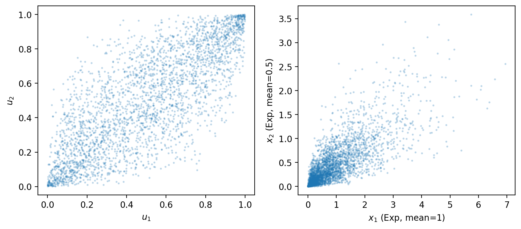
Fig. 8.1 gaussian copula with exponential marginals#
Sample correlation of (x1, x2): 0.768
Sample correlation of (u1, u2): 0.786
The left panel shows the copula itself – the dependence structure in uniform coordinates, drawn from a bivariate normal with correlation \(\rho = 0.8\).
The right panel shows the same dependence translated to exponential marginals.
Changing \(\rho\) controls the strength of dependence while the marginals remain unchanged.
8.17. Exercises#
Exercise 8.1
Independence Test
Consider the joint distribution
where \(X \in \{0,1\}\) and \(Y \in \{10, 20\}\).
Compute the marginal distributions \(\mu_i = \text{Prob}\{X=i\}\) and \(\nu_j = \text{Prob}\{Y=j\}\).
Form the independence matrix \(f^{\perp}_{ij} = \mu_i \nu_j\) (the outer product of the two marginal vectors).
Compare \(F\) with \(f^{\perp}\) and determine whether \(X\) and \(Y\) are independent.
Verify your conclusion by computing \(\text{Prob}\{X=0|Y=10\}\) and checking whether it equals \(\text{Prob}\{X=0\}\).
Solution
Here is one solution:
F = np.array([[0.3, 0.2],
              [0.1, 0.4]])

μ = F.sum(axis=1)
ν = F.sum(axis=0)
print("μ (marginal of X):", μ)
print("ν (marginal of Y):", ν)

F_indep = np.outer(μ, ν)
print("\nIndependence matrix (outer product):\n", F_indep)
print("\nActual joint F:\n", F)

print("\nIndependent (F == μ times ν)?", np.allclose(F, F_indep))

prob_X0_given_Y10 = F[0, 0] / ν[0]
print(f"\nProb(X=0 | Y=10) = {prob_X0_given_Y10:.4f}")
print(f"Prob(X=0)         = {μ[0]:.4f}")
μ (marginal of X): [0.5 0.5]
ν (marginal of Y): [0.4 0.6]

Independence matrix (outer product):
 [[0.2 0.3]
 [0.2 0.3]]

Actual joint F:
 [[0.3 0.2]
 [0.1 0.4]]

Independent (F == μ times ν)? False

Prob(X=0 | Y=10) = 0.7500
Prob(X=0)         = 0.5000
Exercise 8.2
Covariance and Correlation
Using the same joint distribution \(F\) and values \(X \in \{0,1\}\), \(Y \in \{10, 20\}\) as in Exercise 1:
Compute \(\mathbb{E}[X]\), \(\mathbb{E}[Y]\), and \(\mathbb{E}[XY] = \sum_i \sum_j x_i y_j f_{ij}\).
Compute \(\text{Cov}(X,Y) = \mathbb{E}[XY] - \mathbb{E}[X]\mathbb{E}[Y]\).
Compute \(\text{Cor}(X,Y) = \text{Cov}(X,Y) / (\sigma_X \sigma_Y)\).
Show analytically that \(X \perp Y\) implies \(\text{Cov}(X,Y) = 0\).
Solution
Here is one solution:
xs = np.array([0, 1])
ys = np.array([10, 20])
F  = np.array([[0.3, 0.2],
               [0.1, 0.4]])

μ = F.sum(axis=1)
ν = F.sum(axis=0)

E_X  = xs @ μ
E_Y  = ys @ ν
E_XY = sum(xs[i] * ys[j] * F[i, j] for i in range(2) for j in range(2))
print(f"E[X] = {E_X}, E[Y] = {E_Y}, E[XY] = {E_XY}")

cov_XY = E_XY - E_X * E_Y
print(f"Cov(X,Y) = {cov_XY:.4f}")

var_X  = ((xs - E_X)**2) @ μ
var_Y  = ((ys - E_Y)**2) @ ν
cor_XY = cov_XY / np.sqrt(var_X * var_Y)
print(f"Cor(X,Y) = {cor_XY:.4f}")
E[X] = 0.5, E[Y] = 16.0, E[XY] = 9.0
Cov(X,Y) = 1.0000
Cor(X,Y) = 0.4082
For part 4: if \(X \perp Y\) then \(f_{ij} = \mu_i \nu_j\), so
and therefore \(\text{Cov}(X,Y) = \mathbb{E}[XY] - \mathbb{E}[X]\mathbb{E}[Y] = 0\).
Exercise 8.3
Sum of Two Dice
Let \(X\) and \(Y\) be independent random variables, each uniformly distributed on \(\{1,2,3,4,5,6\}\), and let \(Z = X + Y\).
Use the convolution formula \(h_k = \sum_i f_i g_{k-i}\) to compute the distribution of \(Z\).
Plot the result generated by the formula.
Simulate \(10^6\) rolls and overlay the empirical histogram on the plot.
Compute \(\mathbb{E}[Z]\) and \(\text{Var}(Z)\) from the two calculations
Solution
Here is one solution:
f = np.ones(6) / 6
g = np.ones(6) / 6
h = [
    sum(f[i]*g[k-i] for i in range(
        max(0, k-len(g)+1), # f_i exists
        min(len(f), k+1))   # g_{k-i} exists
        )
        for k in range(len(f) + len(g) - 1)]
z_vals = np.arange(2, 13)

n = 1_000_000
z_sim = rng.integers(1, 7, n) + rng.integers(1, 7, n)
counts = np.bincount(z_sim, minlength=13)[2:]

fig, ax = plt.subplots()
ax.bar(z_vals - 0.2, h,          0.4, alpha=0.7, label='Theoretical')
ax.bar(z_vals + 0.2, counts / n, 0.4, alpha=0.7, label='Empirical')
ax.set_xlabel('Z = X + Y')
ax.set_ylabel('Probability')
ax.legend()
plt.show()

E_Z   = z_vals @ h
Var_Z = ((z_vals - E_Z)**2) @ h
print(f"Theory:     E[Z] = {E_Z:.2f}, Var(Z) = {Var_Z:.4f}")
print(f"Simulation: E[Z] = {np.mean(z_sim):.2f}, Var(Z) = {np.var(z_sim):.4f}")
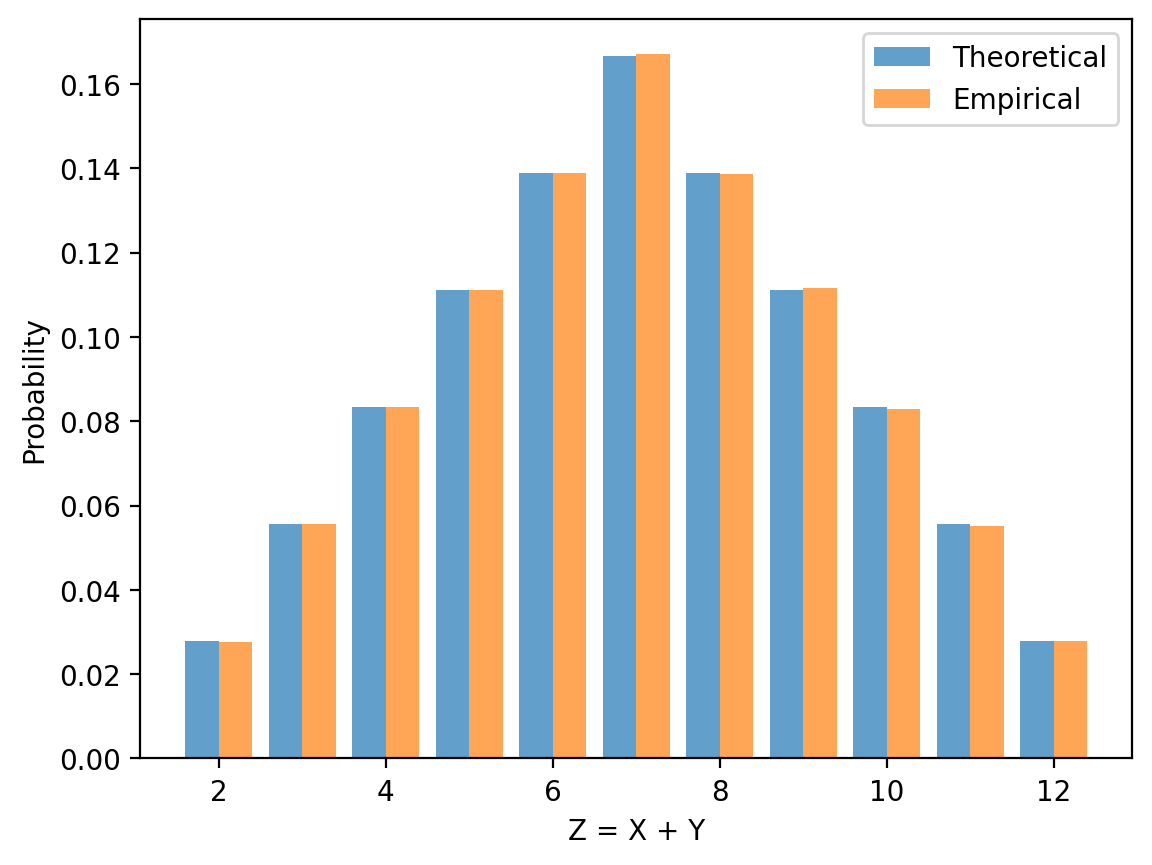
Theory:     E[Z] = 7.00, Var(Z) = 5.8333
Simulation: E[Z] = 7.00, Var(Z) = 5.8271
Exercise 8.4
Multi-Step Transition Probabilities
Consider a two-state Markov chain with transition matrix
where \(p_{ij} = \text{Prob}\{X(t+1)=j \mid X(t)=i\}\).
Starting from \(\psi_0 = [1, 0]\), compute \(\psi_n = \psi_0 P^n\) for \(n = 1, 5, 20, 100\).
Find the stationary distribution \(\psi^*\) satisfying \(\psi^* P = \psi^*\) and \(\sum_i \psi^*_i = 1\).
Verify numerically that \(\psi_n \to \psi^*\) as \(n\) grows.
Solution
Here is one solution:
P = np.array([[0.9, 0.1],
              [0.2, 0.8]])
ψ0 = np.array([1.0, 0.0])

for n in [1, 5, 20, 100]:
    print(f"ψ_{n:3d} = {ψ0 @ np.linalg.matrix_power(P, n)}")

A = np.vstack([P.T - np.eye(2), np.ones(2)])
b = np.array([0.0, 0.0, 1.0])
ψ_star, *_ = np.linalg.lstsq(A, b, rcond=None)
print(f"\nStationary distribution: {ψ_star}")

ψ_100 = ψ0 @ np.linalg.matrix_power(P, 100)
print(f"ψ_100 close to stationary? {np.allclose(ψ_100, ψ_star, atol=1e-6)}")
ψ_  1 = [0.9 0.1]
ψ_  5 = [0.72269 0.27731]
ψ_ 20 = [0.66693264 0.33306736]
ψ_100 = [0.66666667 0.33333333]

Stationary distribution: [0.66666667 0.33333333]
ψ_100 close to stationary? True
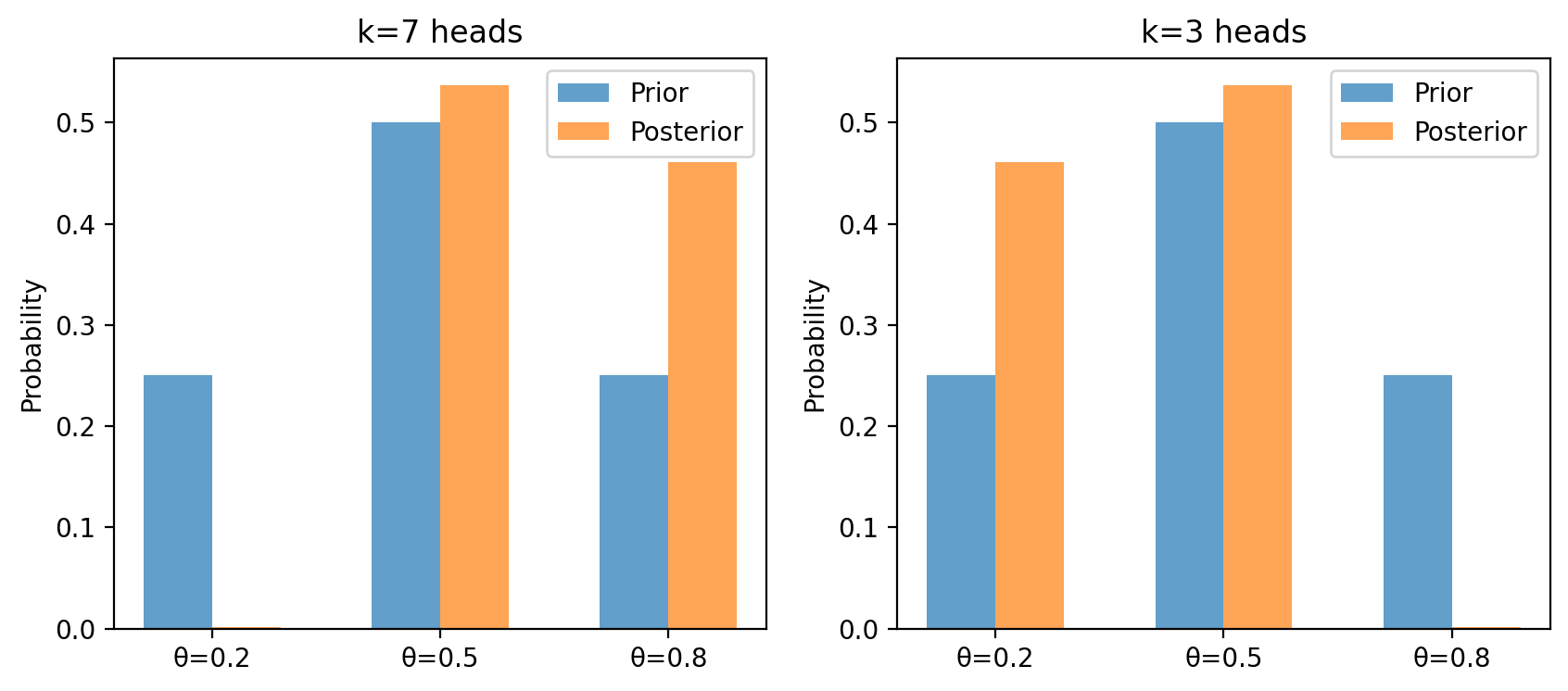
Exercise 8.5
Bayes’ Law with a Discrete Prior
A coin has unknown bias \(\theta \in \{0.2,\, 0.5,\, 0.8\}\) with prior \(\pi = [0.25,\, 0.50,\, 0.25]\).
Assume that, conditional on \(\theta\), the coin flips are i.i.d. Bernoulli(\(\theta\)).
After observing \(k = 7\) heads in \(n = 10\) flips, compute the likelihood
\[ \mathcal{L}(\theta \mid \text{data}) = \binom{10}{7}\,\theta^7\,(1-\theta)^3 \]for each \(\theta\).
Apply equation (8.4) to compute the posterior \(\pi(\theta \mid \text{data})\).
Plot the prior and posterior side by side.
Repeat for \(k = 3\) heads and describe how the posterior shifts.
Solution
Here is one solution:
θ_vals = np.array([0.2, 0.5, 0.8])
π = np.array([0.25, 0.50, 0.25])

def compute_posterior(k, n, θ_vals, π):
    likelihood = comb(n, k) * θ_vals**k * (1 - θ_vals)**(n - k)
    unnorm = likelihood * π
    return unnorm / unnorm.sum(), likelihood

post7, lik7 = compute_posterior(7, 10, θ_vals, π)
post3, lik3 = compute_posterior(3, 10, θ_vals, π)

print("k=7:  likelihood =", lik7.round(4),
      " posterior =", post7.round(4))
print("k=3:  likelihood =", lik3.round(4),
      " posterior =", post3.round(4))

x = np.arange(len(θ_vals))
w = 0.3
fig, axes = plt.subplots(1, 2, figsize=(10, 4))
for ax, post, title in zip(
    axes, [post7, post3], ['k=7 heads', 'k=3 heads']):
    ax.bar(x - w/2, π, w, label='Prior',     alpha=0.7)
    ax.bar(x + w/2, post,  w, label='Posterior', alpha=0.7)
    ax.set_xticks(x)
    ax.set_xticklabels([f'θ={t}' for t in θ_vals])
    ax.set_ylabel('Probability')
    ax.set_title(title)
    ax.legend()
plt.show()
k=7:  likelihood = [0.0008 0.1172 0.2013]  posterior = [0.0018 0.537  0.4612]
k=3:  likelihood = [0.2013 0.1172 0.0008]  posterior = [0.4612 0.537  0.0018]