33. Bayesian versus Frequentist Decision Rules#
import matplotlib.pyplot as plt
import numpy as np
from numba import jit, prange, float64, int64
from numba.experimental import jitclass
from math import gamma
from scipy.optimize import minimize
33.1. Overview#
This lecture follows up on ideas presented in the following lectures:
A Problem that Stumped Milton Friedman described a problem that a Navy Captain presented to Milton Friedman during World War II.
The Navy had told the Captain to use a decision rule for quality control.
In particular, the Navy had ordered the Captain to use an instance of a frequentist decision rule.
The Captain doubted that that rule was a good one.
Milton Friedman recognized the Captain’s conjecture as posing a challenging statistical problem that he and other members of the US Government’s Statistical Research Group at Columbia University proceeded to try to solve.
A member of the group, the great mathematician and economist Abraham Wald, soon solved the problem.
A good way to formulate the problem is to use some ideas from Bayesian statistics that we describe in this lecture Exchangeability and Bayesian Updating and in this lecture Likelihood Ratio Processes, which describes the link between Bayesian updating and likelihood ratio processes.
The present lecture uses Python to generate simulations that evaluate expected losses under the Neyman-Pearson frequentist procedure that the Navy captain questioned and the Bayesian decision rule described in A Bayesian Formulation of Friedman and Wald’s Problem.
The simulations confirm the Navy Captain’s hunch that there is a better rule than the Neyman-Pearson likelihood ratio test that the Navy had told him to use.
33.2. Setup#
To formalize the problem that had confronted the Navy Captain, we consider a setting with the following parts.
Each period a decision maker draws a non-negative random variable \(Z\). He knows that two probability distributions are possible, \(f_{0}\) and \(f_{1}\), and that which ever distribution it is remains fixed over time. The decision maker believes that before the beginning of time, nature once and for all had selected either \(f_{0}\) or \(f_1\) and that the probability that it selected \(f_0\) is probability \(\pi^{*}\).
The decision maker observes a sample \(\left\{ z_{i}\right\} _{i=0}^{t}\) from the distribution chosen by nature.
The decision maker wants to decide which distribution actually governs \(Z\).
He is worried about two types of errors and the losses that they will impose on him.
a loss \(\bar L_{1}\) from a type I error that occurs if he decides that \(f=f_{1}\) when actually \(f=f_{0}\)
a loss \(\bar L_{0}\) from a type II error that occurs if he decides that \(f=f_{0}\) when actually \(f=f_{1}\)
The decision maker pays a cost \(c\) for drawing another \(z\).
We mainly borrow parameters from the quantecon lecture A Bayesian Formulation of Friedman and Wald’s Problem except that we increase both \(\bar L_{0}\) and \(\bar L_{1}\) from \(25\) to \(100\) to encourage the Bayesian decision rule to take more draws before deciding.
We set the cost \(c\) of taking one more draw at \(1.25\).
We set the probability distributions \(f_{0}\) and \(f_{1}\) to be beta distributions with \(a_{0}=b_{0}=1\), \(a_{1}=3\), and \(b_{1}=1.2\), respectively.
Below is some Python code that sets up these objects.
@jit
def p(x, a, b):
    "Beta distribution."

    r = gamma(a + b) / (gamma(a) * gamma(b))

    return r * x**(a-1) * (1 - x)**(b-1)
We start with defining a jitclass that stores parameters and
functions we need to solve problems for both the Bayesian and
frequentist Navy Captains.
wf_data = [
    ('c', float64),           # unemployment compensation
    ('a0', float64),          # parameters of beta distribution
    ('b0', float64),
    ('a1', float64),
    ('b1', float64),
    ('L0', float64),          # cost of selecting f0 when f1 is true
    ('L1', float64),          # cost of selecting f1 when f0 is true
    ('π_grid', float64[:]),   # grid of beliefs π
    ('π_grid_size', int64),
    ('mc_size', int64),       # size of Monto Carlo simulation
    ('z0', float64[:]),       # sequence of random values
    ('z1', float64[:])        # sequence of random values
]
@jitclass(wf_data)
class WaldFriedman:

    def __init__(self,
                 c=1.25,
                 a0=1,
                 b0=1,
                 a1=3,
                 b1=1.2,
                 L0=100,
                 L1=100,
                 π_grid_size=200,
                 mc_size=1000):

        self.c, self.π_grid_size = c, π_grid_size
        self.a0, self.b0, self.a1, self.b1 = a0, b0, a1, b1
        self.L0, self.L1 = L0, L1
        self.π_grid = np.linspace(0, 1, π_grid_size)
        self.mc_size = mc_size

        self.z0 = np.random.beta(a0, b0, mc_size)
        self.z1 = np.random.beta(a1, b1, mc_size)

    def f0(self, x):

        return p(x, self.a0, self.b0)

    def f1(self, x):

        return p(x, self.a1, self.b1)

    def κ(self, z, π):
        """
        Updates π using Bayes' rule and the current observation z
        """

        a0, b0, a1, b1 = self.a0, self.b0, self.a1, self.b1

        π_f0, π_f1 = π * p(z, a0, b0), (1 - π) * p(z, a1, b1)
        π_new = π_f0 / (π_f0 + π_f1)

        return π_new
wf = WaldFriedman()

grid = np.linspace(0, 1, 50)

plt.figure()

plt.title("Two Distributions")
plt.plot(grid, wf.f0(grid), lw=2, label="$f_0$")
plt.plot(grid, wf.f1(grid), lw=2, label="$f_1$")

plt.legend()
plt.xlabel("$z$ values")
plt.ylabel("density of $z_k$")

plt.tight_layout()
plt.show()
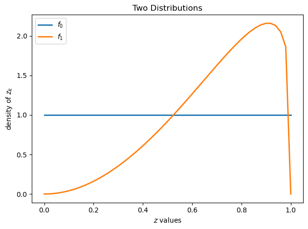
Above, we plot the two possible probability densities \(f_0\) and \(f_1\)
33.3. Frequentist Decision Rule#
The Navy told the Captain to use a Neyman-Pearson likelihood ratio decision rule.
That decision rule is characterized by
a sample size \(t\), and
a cutoff value \(d\) of a likelihood ratio
Let \(L\left(z^{t}\right)=\prod_{i=0}^{t}\frac{f_{0}\left(z_{i}\right)}{f_{1}\left(z_{i}\right)}\) be the likelihood ratio associated with observing the sequence \(\left\{ z_{i}\right\} _{i=0}^{t}\).
The decision rule associated with a sample size \(t\) is:
decide that \(f_0\) is the distribution if the likelihood ratio is greater than \(d\)
decide that \(f_1\) is the distribution if the likelihood ratio is less than \(d\)
For our purposes here, we want to compute an expected loss from using this rule, where we borrow
loss parameters \(\bar L_1\) and \(\bar L_2\) from A Bayesian Formulation of Friedman and Wald’s Problem.
Let null and alternative hypotheses be
null: \(H_{0}\): \(f=f_{0}\),
alternative \(H_{1}\): \(f=f_{1}\).
Given sample size \(t\) and cutoff \(d\), under the model described above, the mathematical expectation of total loss is
Here
\(PFA\) denotes the probability of a false alarm, i.e., rejecting \(H_0\) when it is true
\(PD\) denotes the probability of a detection error, i.e., not rejecting \(H_0\) when \(H_1\) is true
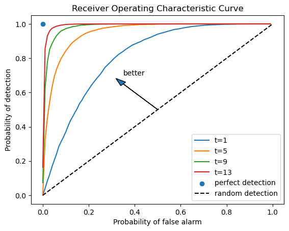
For a given sample size \(t\), the pairs \(\left(PFA,PD\right)\) lie on a receiver operating characteristic curve.
by choosing \(d\), we select a particular pair \(\left(PFA,PD\right)\) along the curve for a given \(t\)
To see some receiver operating characteristic curves, please see this lecture Likelihood Ratio Processes.
To solve for \(\bar{V}_{fre}\left(t,d\right)\) numerically, we first simulate sequences of \(z\) when either \(f_0\) or \(f_1\) generates data.
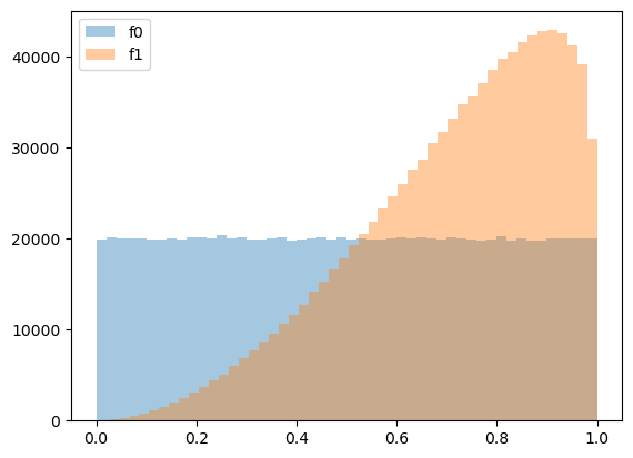
Let’s plot empirical distributions, i.e., histograms, associated with \(f_0\) and \(f_1\).
N = 10000
T = 100
z0_arr = np.random.beta(wf.a0, wf.b0, (N, T))
z1_arr = np.random.beta(wf.a1, wf.b1, (N, T))
plt.hist(z0_arr.flatten(), bins=50, alpha=0.4, label='f0')
plt.hist(z1_arr.flatten(), bins=50, alpha=0.4, label='f1')
plt.legend()
plt.show()
We can compute sequences of likelihood ratios using simulated samples.
l = lambda z: wf.f0(z) / wf.f1(z)
l0_arr = l(z0_arr)
l1_arr = l(z1_arr)

L0_arr = np.cumprod(l0_arr, 1)
L1_arr = np.cumprod(l1_arr, 1)
With an empirical distribution of likelihood ratios in hand, we can draw receiver operating characteristic curves by enumerating \(\left(PFA,PD\right)\) pairs given each sample size \(t\).
PFA = np.arange(0, 100, 1)

for t in range(1, 15, 4):
    percentile = np.percentile(L0_arr[:, t], PFA)
    PD = [np.sum(L1_arr[:, t] < p) / N for p in percentile]

    plt.plot(PFA / 100, PD, label=f"t={t}")

plt.scatter(0, 1, label="perfect detection")
plt.plot([0, 1], [0, 1], color='k', ls='--', label="random detection")

plt.arrow(0.5, 0.5, -0.15, 0.15, head_width=0.03)
plt.text(0.35, 0.7, "better")
plt.xlabel("Probability of false alarm")
plt.ylabel("Probability of detection")
plt.legend()
plt.title("Receiver Operating Characteristic Curve")
plt.show()
We can minimize the expected total loss presented in equation (33.1) by choosing \(\left(t,d\right)\).
Doing that delivers an expected loss
We first consider the case in which \(\pi^{*}=\Pr\left\{ \text{nature selects }f_{0}\right\} =0.5\).
We can solve the minimization problem in two steps.
First, we fix \(t\) and find the optimal cutoff \(d\) and consequently the minimal \(\bar{V}_{fre}\left(t\right)\).
Here is Python code that does that and then plots a useful graph.
@jit
def V_fre_d_t(d, t, L0_arr, L1_arr, π_star, wf):

    N = L0_arr.shape[0]

    PFA = np.sum(L0_arr[:, t-1] < d) / N
    PD = np.sum(L1_arr[:, t-1] < d) / N

    V = π_star * PFA * wf.L1 + (1 - π_star) * (1 - PD) * wf.L0

    return V
def V_fre_t(t, L0_arr, L1_arr, π_star, wf):

    res = minimize(V_fre_d_t, 1, args=(t, L0_arr, L1_arr, π_star, wf), method='Nelder-Mead')
    V = res.fun
    d = res.x

    PFA = np.sum(L0_arr[:, t-1] < d) / N
    PD = np.sum(L1_arr[:, t-1] < d) / N

    return V, PFA, PD
def compute_V_fre(L0_arr, L1_arr, π_star, wf):

    T = L0_arr.shape[1]

    V_fre_arr = np.empty(T)
    PFA_arr = np.empty(T)
    PD_arr = np.empty(T)

    for t in range(1, T+1):
        V, PFA, PD = V_fre_t(t, L0_arr, L1_arr, π_star, wf)
        V_fre_arr[t-1] = wf.c * t + V
        PFA_arr[t-1] = PFA
        PD_arr[t-1] = PD

    return V_fre_arr, PFA_arr, PD_arr
π_star = 0.5
V_fre_arr, PFA_arr, PD_arr = compute_V_fre(L0_arr, L1_arr, π_star, wf)

plt.plot(range(T), V_fre_arr, label=r'$\min_{d} \overline{V}_{fre}(t,d)$')
plt.xlabel('t')
plt.title(r'$\pi^*=0.5$')
plt.legend()
plt.show()
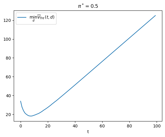
t_optimal = np.argmin(V_fre_arr) + 1
The above graph illustrates how minimizing over \(t\) tells the frequentist to draw \(t_{\rm optimal}\) observations and then decide.
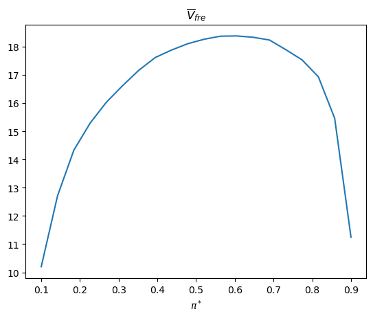
Let’s now change the value of \(\pi^{*}\) and watch how the decision rule changes.
n_π = 20
π_star_arr = np.linspace(0.1, 0.9, n_π)

V_fre_bar_arr = np.empty(n_π)
t_optimal_arr = np.empty(n_π)
PFA_optimal_arr = np.empty(n_π)
PD_optimal_arr = np.empty(n_π)

for i, π_star in enumerate(π_star_arr):
    V_fre_arr, PFA_arr, PD_arr = compute_V_fre(L0_arr, L1_arr, π_star, wf)
    t_idx = np.argmin(V_fre_arr)

    V_fre_bar_arr[i] = V_fre_arr[t_idx]
    t_optimal_arr[i] = t_idx + 1
    PFA_optimal_arr[i] = PFA_arr[t_idx]
    PD_optimal_arr[i] = PD_arr[t_idx]
plt.plot(π_star_arr, V_fre_bar_arr)
plt.xlabel(r'$\pi^*$')
plt.title(r'$\overline{V}_{fre}$')

plt.show()
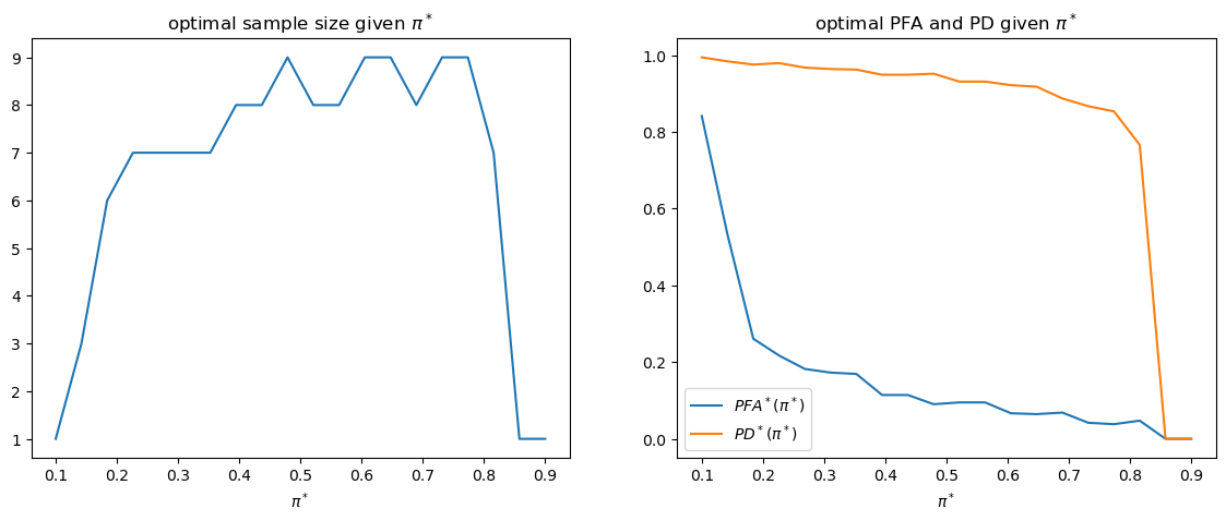
The following shows how optimal sample size \(t\) and targeted \(\left(PFA,PD\right)\) change as \(\pi^{*}\) varies.
fig, axs = plt.subplots(1, 2, figsize=(14, 5))

axs[0].plot(π_star_arr, t_optimal_arr)
axs[0].set_xlabel(r'$\pi^*$')
axs[0].set_title(r'optimal sample size given $\pi^*$')

axs[1].plot(π_star_arr, PFA_optimal_arr, label=r'$PFA^*(\pi^*)$')
axs[1].plot(π_star_arr, PD_optimal_arr, label=r'$PD^*(\pi^*)$')
axs[1].set_xlabel(r'$\pi^*$')
axs[1].legend()
axs[1].set_title(r'optimal PFA and PD given $\pi^*$')

plt.show()
33.4. Bayesian Decision Rule#
In A Problem that Stumped Milton Friedman, we learned how Abraham Wald confirmed the Navy Captain’s hunch that there is a better decision rule.
In A Bayesian Formulation of Friedman and Wald’s Problem we presented a Bayesian procedure that makes decisions by comparing a Bayesian posterior probability \(\pi\) with cutoff probabilities called \(A\) and \(B\).
To proceed, we borrow some Python code from the quantecon lecture A Bayesian Formulation of Friedman and Wald’s Problem that computes optimal values of \(A\) and \(B\).
@jit(parallel=True)
def Q(h, wf):

    c, π_grid = wf.c, wf.π_grid
    L0, L1 = wf.L0, wf.L1
    z0, z1 = wf.z0, wf.z1
    mc_size = wf.mc_size

    κ = wf.κ

    h_new = np.empty_like(π_grid)
    h_func = lambda p: np.interp(p, π_grid, h)

    for i in prange(len(π_grid)):
        π = π_grid[i]

        # Find the expected value of J by integrating over z
        integral_f0, integral_f1 = 0, 0
        for m in range(mc_size):
            π_0 = κ(z0[m], π)  # Draw z from f0 and update π
            integral_f0 += min((1 - π_0) * L0, π_0 * L1, h_func(π_0))

            π_1 = κ(z1[m], π)  # Draw z from f1 and update π
            integral_f1 += min((1 - π_1) * L0, π_1 * L1, h_func(π_1))

        integral = (π * integral_f0 + (1 - π) * integral_f1) / mc_size

        h_new[i] = c + integral

    return h_new
@jit
def solve_model(wf, tol=1e-4, max_iter=1000):
    """
    Compute the continuation value function

    * wf is an instance of WaldFriedman
    """

    # Set up loop
    h = np.zeros(len(wf.π_grid))
    i = 0
    error = tol + 1

    while i < max_iter and error > tol:
        h_new = Q(h, wf)
        error = np.max(np.abs(h - h_new))
        i += 1
        h = h_new

    if error > tol:
        print("Failed to converge!")

    return h_new
h_star = solve_model(wf)
@jit
def find_cutoff_rule(wf, h):

    """
    This function takes a continuation value function and returns the
    corresponding cutoffs of where you transition between continuing and
    choosing a specific model
    """

    π_grid = wf.π_grid
    L0, L1 = wf.L0, wf.L1

    # Evaluate cost at all points on grid for choosing a model
    payoff_f0 = (1 - π_grid) * L0
    payoff_f1 = π_grid * L1

    # The cutoff points can be found by differencing these costs with
    # The Bellman equation (J is always less than or equal to p_c_i)
    B = π_grid[np.searchsorted(
                              payoff_f1 - np.minimum(h, payoff_f0),
                              1e-10)
               - 1]
    A = π_grid[np.searchsorted(
                              np.minimum(h, payoff_f1) - payoff_f0,
                              1e-10)
               - 1]

    return (B, A)

B, A = find_cutoff_rule(wf, h_star)
cost_L0 = (1 - wf.π_grid) * wf.L0
cost_L1 = wf.π_grid * wf.L1

fig, ax = plt.subplots(figsize=(10, 6))

ax.plot(wf.π_grid, h_star, label='continuation value')
ax.plot(wf.π_grid, cost_L1, label='choose f1')
ax.plot(wf.π_grid, cost_L0, label='choose f0')
ax.plot(wf.π_grid,
        np.amin(np.column_stack([h_star, cost_L0, cost_L1]),axis=1),
        lw=15, alpha=0.1, color='b', label='minimum cost')

ax.annotate(r"$B$", xy=(B + 0.01, 0.5), fontsize=14)
ax.annotate(r"$A$", xy=(A + 0.01, 0.5), fontsize=14)

plt.vlines(B, 0, B * wf.L0, linestyle="--")
plt.vlines(A, 0, (1 - A) * wf.L1, linestyle="--")

ax.set(xlim=(0, 1), ylim=(0, 0.5 * max(wf.L0, wf.L1)), ylabel="cost",
       xlabel=r"$\pi$", title="Value function")

plt.legend(borderpad=1.1)
plt.show()
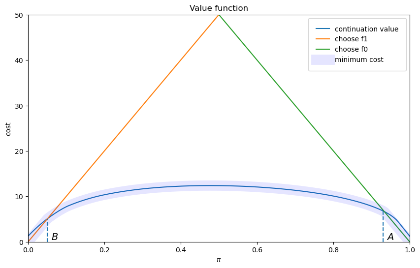
The above figure portrays the value function plotted against the decision maker’s Bayesian posterior.
It also shows the cutoff probabilities \(A\) and \(B\).
The Bayesian decision rule is:
accept \(H_0\) if \(\pi \geq A\)
accept \(H_1\) if \(\pi \leq B\)
delay deciding and draw another \(z\) if \( B \leq \pi \leq A\)
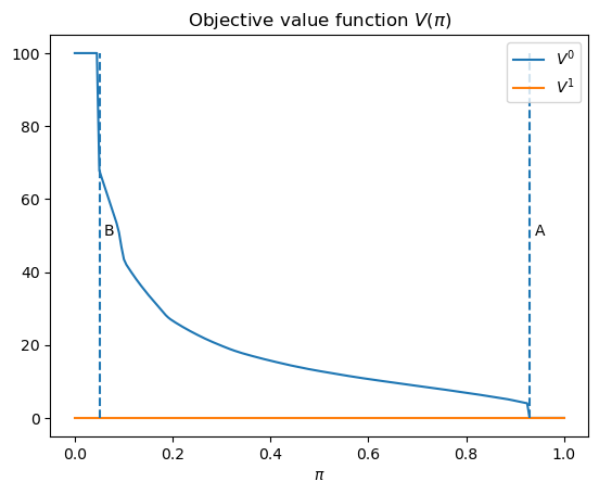
We can calculate two “objective” loss functions under this situation conditioning on knowing for sure that nature has selected \(f_{0}\), in the first case, or \(f_{1}\), in the second case.
under \(f_{0}\),
\[\begin{split} V^{0}\left(\pi\right)=\begin{cases} 0 & \text{if} A \leq\pi,\\ c+EV^{0}\left(\pi^{\prime}\right) & \text{if }B\leq\pi< A,\\ \bar L_{1} & \text{if }\pi<B. \end{cases} \end{split}\]under \(f_{1}\)
\[\begin{split} V^{1}\left(\pi\right)=\begin{cases} \bar L_{0} & \text{if }A \leq\pi,\\ c+EV^{1}\left(\pi^{\prime}\right) & \text{if }B \leq\pi<A,\\ 0 & \text{if }\pi< B. \end{cases} \end{split}\]
where \(\pi^{\prime}=\frac{\pi f_{0}\left(z^{\prime}\right)}{\pi f_{0}\left(z^{\prime}\right)+\left(1-\pi\right)f_{1}\left(z^{\prime}\right)}\).
Given a prior probability \(\pi_{0}\), the expected loss for the Bayesian is
Below we write some Python code that computes \(V^{0}\left(\pi\right)\) and \(V^{1}\left(\pi\right)\) numerically.
@jit(parallel=True)
def V_q(wf, flag):
    V = np.zeros(wf.π_grid_size)
    if flag == 0:
        z_arr = wf.z0
        V[wf.π_grid < B] = wf.L1
    else:
        z_arr = wf.z1
        V[wf.π_grid >= A] = wf.L0

    V_old = np.empty_like(V)

    while True:
        V_old[:] = V[:]
        V[(B <= wf.π_grid) & (wf.π_grid < A)] = 0

        for i in prange(len(wf.π_grid)):
            π = wf.π_grid[i]

            if π >= A or π < B:
                continue

            for j in prange(len(z_arr)):
                π_next = wf.κ(z_arr[j], π)
                V[i] += wf.c + np.interp(π_next, wf.π_grid, V_old)

            V[i] /= wf.mc_size

        if np.abs(V - V_old).max() < 1e-5:
            break

    return V
V0 = V_q(wf, 0)
V1 = V_q(wf, 1)

plt.plot(wf.π_grid, V0, label='$V^0$')
plt.plot(wf.π_grid, V1, label='$V^1$')
plt.vlines(B, 0, wf.L0, linestyle='--')
plt.text(B+0.01, wf.L0/2, 'B')
plt.vlines(A, 0, wf.L0, linestyle='--')
plt.text(A+0.01, wf.L0/2, 'A')
plt.xlabel(r'$\pi$')
plt.title(r'Objective value function $V(\pi)$')
plt.legend()
plt.show()
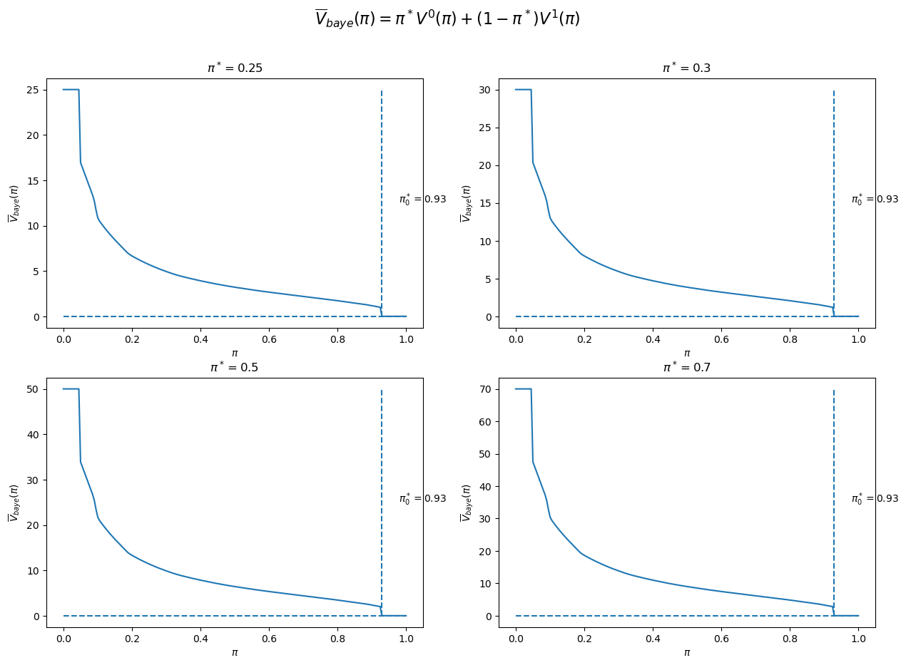
Given an assumed value for \(\pi^{*}=\Pr\left\{ \text{nature selects }f_{0}\right\}\), we can then compute \(\bar{V}_{Bayes}\left(\pi_{0}\right)\).
We can then determine an initial Bayesian prior \(\pi_{0}^{*}\) that minimizes this objective concept of expected loss.
The figure below plots four cases corresponding to \(\pi^{*}=0.25,0.3,0.5,0.7\).
We observe that in each case \(\pi_{0}^{*}\) equals \(\pi^{*}\).
def compute_V_baye_bar(π_star, V0, V1, wf):

    V_baye = π_star * V0 + (1 - π_star) * V1
    π_idx = np.argmin(V_baye)
    π_optimal = wf.π_grid[π_idx]
    V_baye_bar = V_baye[π_idx]

    return V_baye, π_optimal, V_baye_bar
π_star_arr = [0.25, 0.3, 0.5, 0.7]

fig, axs = plt.subplots(2, 2, figsize=(15, 10))

for i, π_star in enumerate(π_star_arr):
    row_i = i // 2
    col_i = i % 2

    V_baye, π_optimal, V_baye_bar = compute_V_baye_bar(π_star, V0, V1, wf)

    axs[row_i, col_i].plot(wf.π_grid, V_baye)
    axs[row_i, col_i].hlines(V_baye_bar, 0, 1, linestyle='--')
    axs[row_i, col_i].vlines(π_optimal, V_baye_bar, V_baye.max(), linestyle='--')
    axs[row_i, col_i].text(π_optimal+0.05, (V_baye_bar + V_baye.max()) / 2,
                        r'${\pi_0^*}=$'+f'{π_optimal:0.2f}')
    axs[row_i, col_i].set_xlabel(r'$\pi$')
    axs[row_i, col_i].set_ylabel(r'$\overline{V}_{baye}(\pi)$')
    axs[row_i, col_i].set_title(r'$\pi^*=$' + f'{π_star}')

fig.suptitle(r'$\overline{V}_{baye}(\pi)=\pi^*V^0(\pi) + (1-\pi^*)V^1(\pi)$', fontsize=16)
plt.show()
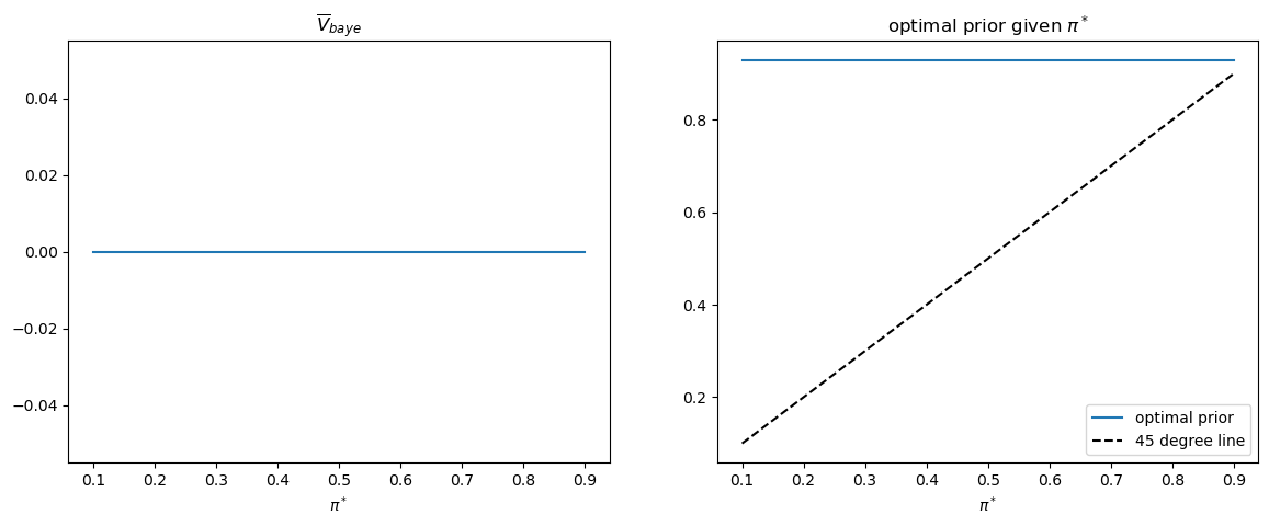
This pattern of outcomes holds more generally.
Thus, the following Python code generates the associated graph that verifies the equality of \(\pi_{0}^{*}\) to \(\pi^{*}\) holds for all \(\pi^{*}\).
π_star_arr = np.linspace(0.1, 0.9, n_π)
V_baye_bar_arr = np.empty_like(π_star_arr)
π_optimal_arr = np.empty_like(π_star_arr)

for i, π_star in enumerate(π_star_arr):

    V_baye, π_optimal, V_baye_bar = compute_V_baye_bar(π_star, V0, V1, wf)

    V_baye_bar_arr[i] = V_baye_bar
    π_optimal_arr[i] = π_optimal

fig, axs = plt.subplots(1, 2, figsize=(14, 5))

axs[0].plot(π_star_arr, V_baye_bar_arr)
axs[0].set_xlabel(r'$\pi^*$')
axs[0].set_title(r'$\overline{V}_{baye}$')

axs[1].plot(π_star_arr, π_optimal_arr, label='optimal prior')
axs[1].plot([π_star_arr.min(), π_star_arr.max()],
            [π_star_arr.min(), π_star_arr.max()],
            c='k', linestyle='--', label='45 degree line')
axs[1].set_xlabel(r'$\pi^*$')
axs[1].set_title(r'optimal prior given $\pi^*$')
axs[1].legend()

plt.show()
33.5. Was the Navy Captain’s Hunch Correct?#
We now compare average losses obtained by our frequentist Neyman-Pearson and Bayesian decision rules.
As a starting point, let’s compare average loss functions when \(\pi^{*}=0.5\).
π_star = 0.5
# frequentist
V_fre_arr, PFA_arr, PD_arr = compute_V_fre(L0_arr, L1_arr, π_star, wf)

# bayesian
V_baye = π_star * V0 + (1 - π_star) * V1
V_baye_bar = V_baye.min()
plt.plot(range(T), V_fre_arr, label=r'$\min_{d} \overline{V}_{fre}(t,d)$')
plt.plot([0, T], [V_baye_bar, V_baye_bar], label=r'$\overline{V}_{baye}$')
plt.xlabel('t')
plt.title(r'$\pi^*=0.5$')
plt.legend()
plt.show()
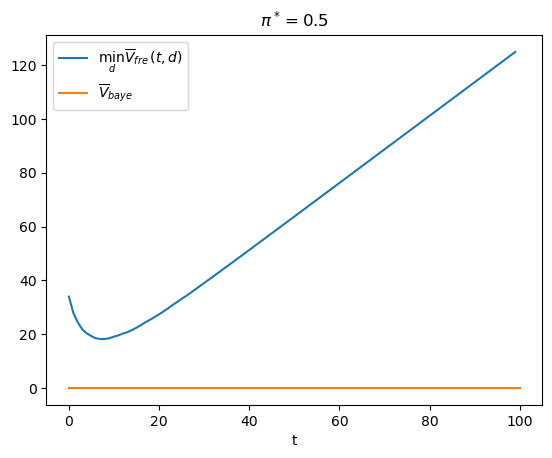
Evidently, there is no sample size \(t\) at which the Neyman-Pearson decision rule attains a lower loss function than does the Bayesian rule.
Furthermore, the following graph indicates that the Bayesian decision rule does better on average for all values of \(\pi^{*}\).
fig, axs = plt.subplots(1, 2, figsize=(14, 5))

axs[0].plot(π_star_arr, V_fre_bar_arr, label=r'$\overline{V}_{fre}$')
axs[0].plot(π_star_arr, V_baye_bar_arr, label=r'$\overline{V}_{baye}$')
axs[0].legend()
axs[0].set_xlabel(r'$\pi^*$')

axs[1].plot(π_star_arr, V_fre_bar_arr - V_baye_bar_arr, label='$diff$')
axs[1].legend()
axs[1].set_xlabel(r'$\pi^*$')

plt.show()
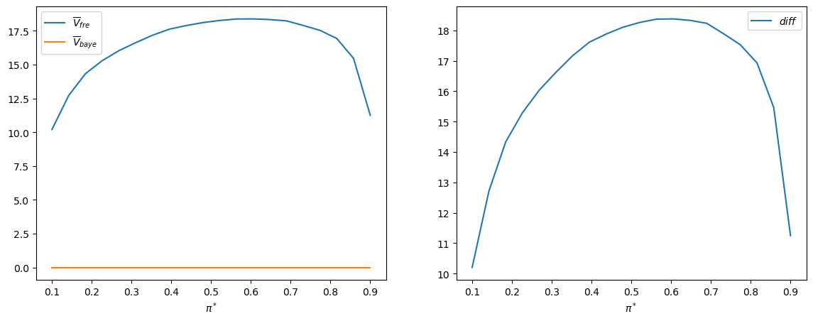
The right panel of the above graph plots the difference \(\bar{V}_{fre}-\bar{V}_{Bayes}\).
It is always positive.
33.6. More Details#
We can provide more insights by focusing on the case in which \(\pi^{*}=0.5=\pi_{0}\).
π_star = 0.5
Recall that when \(\pi^*=0.5\), the frequentist Neyman-Pearson decision rule sets a
sample size t_optimal ex ante.
For our parameter settings, we can compute its value:
t_optimal
np.int64(9)
For convenience, let’s define t_idx as the Python array index
corresponding to t_optimal sample size.
t_idx = t_optimal - 1
33.7. Distribution of Bayesian Decision Rule’s Time to Decide#
We use simulations to compute the frequency distribution of the time to decide for the Bayesian decision rule and compare that time to the frequentist rule’s fixed \(t\).
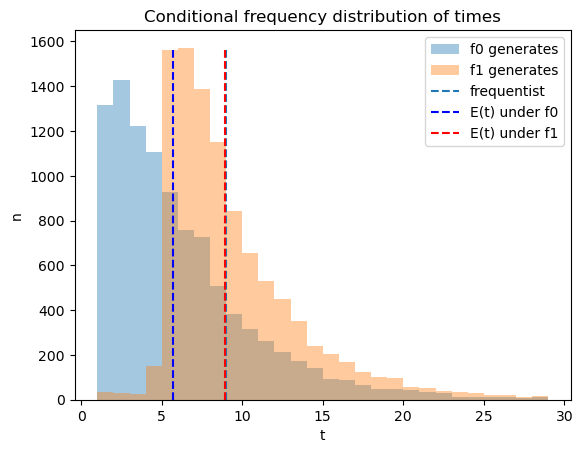
The following Python code creates a graph that shows the frequency distribution of Bayesian times to decide of Bayesian decision maker, conditional on distribution \(q=f_{0}\) or \(q= f_{1}\) generating the data.
The blue and red dotted lines show averages for the Bayesian decision rule, while the black dotted line shows the frequentist optimal sample size \(t\).
On average the Bayesian rule decides earlier than the frequentist rule when \(q= f_0\) and later when \(q = f_1\).
@jit(parallel=True)
def check_results(L_arr, A, B, flag, π0):

    N, T = L_arr.shape

    time_arr = np.empty(N)
    correctness = np.empty(N)

    π_arr = π0 * L_arr / (π0 * L_arr + 1 - π0)

    for i in prange(N):
        for t in range(T):
            if (π_arr[i, t] < B) or (π_arr[i, t] > A):
                time_arr[i] = t + 1
                correctness[i] = (flag == 0 and π_arr[i, t] > A) or (flag == 1 and π_arr[i, t] < B)
                break

    return time_arr, correctness
time_arr0, correctness0 = check_results(L0_arr, A, B, 0, π_star)
time_arr1, correctness1 = check_results(L1_arr, A, B, 1, π_star)

# unconditional distribution
time_arr_u = np.concatenate((time_arr0, time_arr1))
correctness_u = np.concatenate((correctness0, correctness1))
n1 = plt.hist(time_arr0, bins=range(1, 30), alpha=0.4, label='f0 generates')[0]
n2 = plt.hist(time_arr1, bins=range(1, 30), alpha=0.4, label='f1 generates')[0]
plt.vlines(t_optimal, 0, max(n1.max(), n2.max()), linestyle='--', label='frequentist')
plt.vlines(np.mean(time_arr0), 0, max(n1.max(), n2.max()),
           linestyle='--', color='b', label='E(t) under f0')
plt.vlines(np.mean(time_arr1), 0, max(n1.max(), n2.max()),
           linestyle='--', color='r', label='E(t) under f1')
plt.legend();

plt.xlabel('t')
plt.ylabel('n')
plt.title('Conditional frequency distribution of times')

plt.show()
Later we’ll figure out how these distributions ultimately affect objective expected values under the Neyman-Pearson and Bayesian decision rules.
To begin, let’s look at simulations of the Bayesian’s beliefs over time.
We can compute updated beliefs at any time \(t\) using the one-to-one mapping from \(L_{t}\) to \(\pi_{t}\) given \(\pi_0\) described in this lecture Likelihood Ratio Processes.
π0_arr = π_star * L0_arr / (π_star * L0_arr + 1 - π_star)
π1_arr = π_star * L1_arr / (π_star * L1_arr + 1 - π_star)
fig, axs = plt.subplots(1, 2, figsize=(14, 4))

axs[0].plot(np.arange(1, π0_arr.shape[1]+1), np.mean(π0_arr, 0), label='f0 generates')
axs[0].plot(np.arange(1, π1_arr.shape[1]+1), 1 - np.mean(π1_arr, 0), label='f1 generates')
axs[0].set_xlabel('t')
axs[0].set_ylabel(r'$E(\pi_t)$ or ($1 - E(\pi_t)$)')
axs[0].set_title('Expectation of beliefs after drawing t observations')
axs[0].legend()

axs[1].plot(np.arange(1, π0_arr.shape[1]+1), np.var(π0_arr, 0), label='f0 generates')
axs[1].plot(np.arange(1, π1_arr.shape[1]+1), np.var(π1_arr, 0), label='f1 generates')
axs[1].set_xlabel('t')
axs[1].set_ylabel(r'var($\pi_t$)')
axs[1].set_title('Variance of beliefs after drawing t observations')
axs[1].legend()

plt.show()
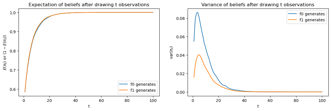
The above figures compare averages and variances of updated Bayesian posteriors after \(t\) draws.
The left graph compares \(E\left(\pi_{t}\right)\) under \(f_{0}\) to \(1-E\left(\pi_{t}\right)\) under \(f_{1}\): they lie on top of each other.
However, as the right hand side graph shows, there is significant difference in variances when \(t\) is small: the variance is lower under \(f_{1}\).
The difference in variances is the reason that the Bayesian decision maker waits longer to decide when \(f_{1}\) generates the data.
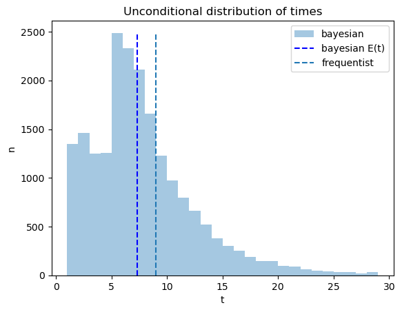
The code below plots outcomes of constructing an unconditional distribution by simply pooling the simulated data across the two possible distributions \(f_0\) and \(f_1\).
The pooled distribution describes a sense in which on average the Bayesian decides earlier, an outcome that seems at least partly to confirm the Navy Captain’s hunch.
n = plt.hist(time_arr_u, bins=range(1, 30), alpha=0.4, label='bayesian')[0]
plt.vlines(np.mean(time_arr_u), 0, n.max(), linestyle='--',
           color='b', label='bayesian E(t)')
plt.vlines(t_optimal, 0, n.max(), linestyle='--', label='frequentist')
plt.legend()

plt.xlabel('t')
plt.ylabel('n')
plt.title('Unconditional distribution of times')

plt.show()
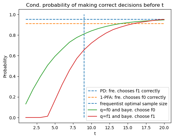
33.8. Probability of Making Correct Decision#
Now we use simulations to compute the fractions of samples in which the Bayesian and the frequentist Neyman-Pearson decision rules decide correctly.
For the frequentist Neyman-Pearson rule, the probability of making the correct decision under \(f_{1}\) is the optimal probability of detection given \(t\) that we defined earlier, and similarly it equals \(1\) minus the optimal probability of a false alarm under \(f_{0}\).
Below we plot these two probabilities for the frequentist rule, along with the conditional probabilities that the Bayesian rule decides before \(t\) and that the decision is correct.
# optimal PFA and PD of frequentist with optimal sample size
V, PFA, PD = V_fre_t(t_optimal, L0_arr, L1_arr, π_star, wf)
plt.plot([1, 20], [PD, PD], linestyle='--', label='PD: fre. chooses f1 correctly')
plt.plot([1, 20], [1-PFA, 1-PFA], linestyle='--', label='1-PFA: fre. chooses f0 correctly')
plt.vlines(t_optimal, 0, 1, linestyle='--', label='frequentist optimal sample size')

N = time_arr0.size
T_arr = np.arange(1, 21)
plt.plot(T_arr, [np.sum(correctness0[time_arr0 <= t] == 1) / N for t in T_arr],
        label='q=f0 and baye. choose f0')
plt.plot(T_arr, [np.sum(correctness1[time_arr1 <= t] == 1) / N for t in T_arr],
        label='q=f1 and baye. choose f1')
plt.legend(loc=4)

plt.xlabel('t')
plt.ylabel('Probability')
plt.title('Cond. probability of making correct decisions before t')

plt.show()
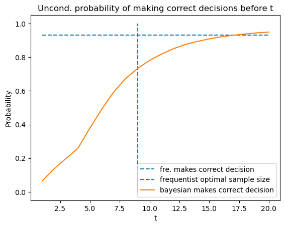
By averaging using \(\pi^{*}\), we also plot the unconditional distribution.
plt.plot([1, 20], [(PD + 1 - PFA) / 2, (PD + 1 - PFA) / 2],
        linestyle='--', label='fre. makes correct decision')
plt.vlines(t_optimal, 0, 1, linestyle='--', label='frequentist optimal sample size')

N = time_arr_u.size
plt.plot(T_arr, [np.sum(correctness_u[time_arr_u <= t] == 1) / N for t in T_arr],
        label="bayesian makes correct decision")
plt.legend()

plt.xlabel('t')
plt.ylabel('Probability')
plt.title('Uncond. probability of making correct decisions before t')

plt.show()
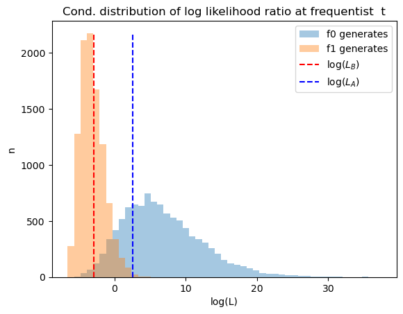
33.9. Distribution of Likelihood Ratios at Neyman-Pearson’s \(t\)#
Next we use simulations to construct distributions of likelihood ratios after \(t\) draws.
To serve as useful reference points, we also show likelihood ratios that correspond to the Bayesian cutoffs \(A\) and \(B\).
In order to exhibit the distribution more clearly, we report logarithms of likelihood ratios.
The graphs below reports two distributions, one conditional on \(f_0\) generating the data, the other conditional on \(f_1\) generating the data.
LA = (1 - π_star) *  A / (π_star - π_star * A)
LB = (1 - π_star) *  B / (π_star - π_star * B)
L_min = min(L0_arr[:, t_idx].min(), L1_arr[:, t_idx].min())
L_max = max(L0_arr[:, t_idx].max(), L1_arr[:, t_idx].max())
bin_range = np.linspace(np.log(L_min), np.log(L_max), 50)
n0 = plt.hist(np.log(L0_arr[:, t_idx]), bins=bin_range, alpha=0.4, label='f0 generates')[0]
n1 = plt.hist(np.log(L1_arr[:, t_idx]), bins=bin_range, alpha=0.4, label='f1 generates')[0]

plt.vlines(np.log(LB), 0, max(n0.max(), n1.max()), linestyle='--', color='r', label='log($L_B$)')
plt.vlines(np.log(LA), 0, max(n0.max(), n1.max()), linestyle='--', color='b', label='log($L_A$)')
plt.legend()

plt.xlabel('log(L)')
plt.ylabel('n')
plt.title('Cond. distribution of log likelihood ratio at frequentist  t')

plt.show()
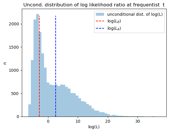
The next graph plots the unconditional distribution of Bayesian times to decide, constructed as earlier by pooling the two conditional distributions.
plt.hist(np.log(np.concatenate([L0_arr[:, t_idx], L1_arr[:, t_idx]])),
        bins=50, alpha=0.4, label='unconditional dist. of log(L)')
plt.vlines(np.log(LB), 0, max(n0.max(), n1.max()), linestyle='--', color='r', label='log($L_B$)')
plt.vlines(np.log(LA), 0, max(n0.max(), n1.max()), linestyle='--', color='b', label='log($L_A$)')
plt.legend()

plt.xlabel('log(L)')
plt.ylabel('n')
plt.title('Uncond. distribution of log likelihood ratio at frequentist  t')

plt.show()