9. Some Probability Distributions#

This lecture is a supplement to this lecture on statistics with matrices.

It describes some popular distributions and uses Python to sample from them.

It also describes a way to sample from an arbitrary probability distribution that you make up by transforming a sample from a uniform probability distribution.

In addition to what’s in Anaconda, this lecture will need the following libraries:

!pip install prettytable

As usual, we’ll start with some imports

import numpy as np
import matplotlib.pyplot as plt
import prettytable as pt
from mpl_toolkits.mplot3d import Axes3D
from matplotlib_inline.backend_inline import set_matplotlib_formats
set_matplotlib_formats('retina')

9.1. Some Discrete Probability Distributions#

Let’s write some Python code to compute means and variances of some univariate random variables.

We’ll use our code to

compute population means and variances from the probability distribution
generate a sample of \(N\) independently and identically distributed draws and compute sample means and variances
compare population and sample means and variances

9.2. Geometric distribution#

\[ \textrm{Prob}(X=k)=(1-p)^{k-1}p,k=1,2, \ldots \]

\(\implies\)

\[\begin{split} \begin{aligned} \mathbb{E}(X) & =\frac{1}{p}\\\mathbb{D}(X) & =\frac{1-p}{p^2} \end{aligned} \end{split}\]

We draw observations from the distribution and compare the sample mean and variance with the theoretical results.

# specify parameters
p, n = 0.3, 1_000_000

# draw observations from the distribution
x = np.random.geometric(p, n)

# compute sample mean and variance
μ_hat = np.mean(x)
σ2_hat = np.var(x)

print("The sample mean is: ", μ_hat, "\nThe sample variance is: ", σ2_hat)

# compare with theoretical results
print("\nThe population mean is: ", 1/p)
print("The population variance is: ", (1-p)/(p**2))

The sample mean is:  3.332628 
The sample variance is:  7.782876613616006

The population mean is:  3.3333333333333335
The population variance is:  7.777777777777778

9.3. Pascal (negative binomial) distribution#

Consider a sequence of independent Bernoulli trials.

Let \(p\) be the probability of success.

Let \(X\) be a random variable that represents the number of failures before we get \(r\) success.

Its distribution is

\[\begin{split} \begin{aligned} X & \sim NB(r,p) \\ \textrm{Prob}(X=k;r,p) & = \begin{pmatrix}k+r-1 \\ r-1 \end{pmatrix}p^r(1-p)^{k} \end{aligned} \end{split}\]

Here, we choose from among \(k+r-1\) possible outcomes because the last draw is by definition a success.

We compute the mean and variance to be

\[\begin{split} \begin{aligned} \mathbb{E}(X) & = \frac{k(1-p)}{p} \\ \mathbb{V}(X) & = \frac{k(1-p)}{p^2} \end{aligned} \end{split}\]

# specify parameters
r, p, n = 10, 0.3, 1_000_000

# draw observations from the distribution
x = np.random.negative_binomial(r, p, n)

# compute sample mean and variance
μ_hat = np.mean(x)
σ2_hat = np.var(x)

print("The sample mean is: ", μ_hat, "\nThe sample variance is: ", σ2_hat)
print("\nThe population mean is: ", r*(1-p)/p)
print("The population variance is: ", r*(1-p)/p**2)

The sample mean is:  23.333182 
The sample variance is:  77.82828375487601

The population mean is:  23.333333333333336
The population variance is:  77.77777777777779

9.4. Newcomb–Benford distribution#

The Newcomb–Benford law fits many data sets, e.g., reports of incomes to tax authorities, in which the leading digit is more likely to be small than large.

See https://en.wikipedia.org/wiki/Benford’s_law

A Benford probability distribution is

\[ \textrm{Prob}\{X=d\}=\log _{10}(d+1)-\log _{10}(d)=\log _{10}\left(1+\frac{1}{d}\right) \]

where \(d\in\{1,2,\cdots,9\}\) can be thought of as a first digit in a sequence of digits.

This is a well defined discrete distribution since we can verify that probabilities are nonnegative and sum to \(1\).

\[ \log_{10}\left(1+\frac{1}{d}\right)\geq0,\quad\sum_{d=1}^{9}\log_{10}\left(1+\frac{1}{d}\right)=1 \]

The mean and variance of a Benford distribution are

\[\begin{split} \begin{aligned} \mathbb{E}\left[X\right] &=\sum_{d=1}^{9}d\log_{10}\left(1+\frac{1}{d}\right)\simeq3.4402 \\ \mathbb{V}\left[X\right] & =\sum_{d=1}^{9}\left(d-\mathbb{E}\left[X\right]\right)^{2}\log_{10}\left(1+\frac{1}{d}\right)\simeq6.0565 \end{aligned} \end{split}\]

We verify the above and compute the mean and variance using numpy.

Benford_pmf = np.array([np.log10(1+1/d) for d in range(1,10)])
k = np.array(range(1,10))

# mean
mean = np.sum(Benford_pmf * k)

# variance
var = np.sum([(k-mean)**2 * Benford_pmf])

# verify sum to 1
print(np.sum(Benford_pmf))
print(mean)
print(var)

0
4402369671232065
056512631375665

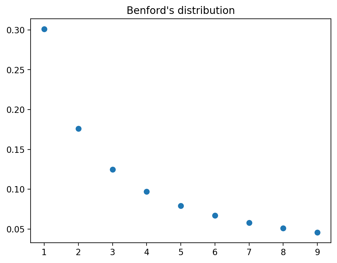
# plot distribution
plt.plot(range(1,10), Benford_pmf, 'o')
plt.title('Benford\'s distribution')
plt.show()

_images/0085ffe51ace5be2b9f5bf6cf450d92603275505637803a0631c3cf0a4751f6c.png

Now let’s turn to some continuous random variables.

9.5. Univariate Gaussian distribution#

We write

\[ X \sim N(\mu,\sigma^2) \]

to indicate the probability distribution

\[f(x|u,\sigma^2)=\frac{1}{\sqrt{2\pi \sigma^2}}e^{[-\frac{1}{2\sigma^2}(x-u)^2]} \]

In the below example, we set \(\mu = 0, \sigma = 0.1\).

# specify parameters
μ, σ = 0, 0.1

# specify number of draws
n = 1_000_000

# draw observations from the distribution
x = np.random.normal(μ, σ, n)

# compute sample mean and variance
μ_hat = np.mean(x)
σ_hat = np.std(x)

print("The sample mean is: ", μ_hat)
print("The sample standard deviation is: ", σ_hat)

The sample mean is:  0.0001255481113103192
The sample standard deviation is:  0.09998344983288851

# compare
print(μ-μ_hat < 1e-3)
print(σ-σ_hat < 1e-3)

True
True

9.6. Uniform Distribution#

\[\begin{split} \begin{aligned} X & \sim U[a,b] \\ f(x)& = \begin{cases} \frac{1}{b-a}, & a \leq x \leq b \\ \quad0, & \text{otherwise} \end{cases} \end{aligned} \end{split}\]

The population mean and variance are

\[\begin{split} \begin{aligned} \mathbb{E}(X) & = \frac{a+b}{2} \\ \mathbb{V}(X) & = \frac{(b-a)^2}{12} \end{aligned} \end{split}\]

# specify parameters
a, b = 10, 20

# specify number of draws
n = 1_000_000

# draw observations from the distribution
x = a + (b-a)*np.random.rand(n)

# compute sample mean and variance
μ_hat = np.mean(x)
σ2_hat = np.var(x)

print("The sample mean is: ", μ_hat, "\nThe sample variance is: ", σ2_hat)
print("\nThe population mean is: ", (a+b)/2)
print("The population variance is: ", (b-a)**2/12)

The sample mean is:  14.996410590435175 
The sample variance is:  8.328531191988626

The population mean is:  15.0
The population variance is:  8.333333333333334

9.7. A Mixed Discrete-Continuous Distribution#

We’ll motivate this example with a little story.

Suppose that to apply for a job you take an interview and either pass or fail it.

You have \(5\%\) chance to pass an interview and you know your salary will uniformly distributed in the interval 300~400 a day only if you pass.

We can describe your daily salary as a discrete-continuous variable with the following probabilities:

\[ P(X=0)=0.95 \]

\[ P(300\le X \le 400)=\int_{300}^{400} f(x)\, dx=0.05 \]

\[ f(x) = 0.0005 \]

Let’s start by generating a random sample and computing sample moments.

x = np.random.rand(1_000_000)
# x[x > 0.95] = 100*x[x > 0.95]+300
x[x > 0.95] = 100*np.random.rand(len(x[x > 0.95]))+300
x[x <= 0.95] = 0

μ_hat = np.mean(x)
σ2_hat = np.var(x)

print("The sample mean is: ", μ_hat, "\nThe sample variance is: ", σ2_hat)

The sample mean is:  17.58392619268439 
The sample variance is:  5890.930767506493

The analytical mean and variance can be computed:

\[\begin{split} \begin{aligned} \mu &= \int_{300}^{400}xf(x)dx \\ &= 0.0005\int_{300}^{400}xdx \\ &= 0.0005 \times \frac{1}{2}x^2\bigg|_{300}^{400} \end{aligned} \end{split}\]

\[\begin{split} \begin{aligned} \sigma^2 &= 0.95\times(0-17.5)^2+\int_{300}^{400}(x-17.5)^2f(x)dx \\ &= 0.95\times17.5^2+0.0005\int_{300}^{400}(x-17.5)^2dx \\ &= 0.95\times17.5^2+0.0005 \times \frac{1}{3}(x-17.5)^3 \bigg|_{300}^{400} \end{aligned} \end{split}\]

mean = 0.0005*0.5*(400**2 - 300**2)
var = 0.95*17.5**2+0.0005/3*((400-17.5)**3-(300-17.5)**3)
print("mean: ", mean)
print("variance: ", var)

mean:  17.5
variance:  5860.416666666666

9.8. Drawing a Random Number from a Particular Distribution#

Suppose we have at our disposal a pseudo random number that draws a uniform random variable, i.e., one with probability distribution

\[ \textrm{Prob}\{\tilde{X}=i\}=\frac{1}{I},\quad i=0,\ldots,I-1 \]

How can we transform \(\tilde{X}\) to get a random variable \(X\) for which \(\textrm{Prob}\{X=i\}=f_i,\quad i=0,\ldots,I-1\), where \(f_i\) is an arbitary discrete probability distribution on \(i=0,1,\dots,I-1\)?

The key tool is the inverse of a cumulative distribution function (CDF).

Observe that the CDF of a distribution is monotone and non-decreasing, taking values between \(0\) and \(1\).

We can draw a sample of a random variable \(X\) with a known CDF as follows:

draw a random variable \(u\) from a uniform distribution on \([0,1]\)
pass the sample value of \(u\) into the “inverse” target CDF for \(X\)
\(X\) has the target CDF

Thus, knowing the “inverse” CDF of a distribution is enough to simulate from this distribution.

Note

The “inverse” CDF needs to exist for this method to work.

The inverse CDF is

\[ F^{-1}(u)\equiv\inf \{x\in \mathbb{R}: F(x) \geq u\} \quad(0<u<1) \]

Here we use infimum because a CDF is a non-decreasing and right-continuous function.

Thus, suppose that

\(U\) is a uniform random variable \(U\in[0,1]\)
We want to sample a random variable \(X\) whose CDF is \(F\).

It turns out that if we use draw uniform random numbers \(U\) and then compute \(X\) from

\[ X=F^{-1}(U), \]

then \(X\) is a random variable with CDF \(F_X(x)=F(x)=\textrm{Prob}\{X\le x\}\).

We’ll verify this in the special case in which \(F\) is continuous and bijective so that its inverse function exists and can be denoted by \(F^{-1}\).

Note that

\[\begin{split} \begin{aligned} F_{X}\left(x\right) & =\textrm{Prob}\left\{ X\leq x\right\} \\ & =\textrm{Prob}\left\{ F^{-1}\left(U\right)\leq x\right\} \\ & =\textrm{Prob}\left\{ U\leq F\left(x\right)\right\} \\ & =F\left(x\right) \end{aligned} \end{split}\]

where the last equality occurs because \(U\) is distributed uniformly on \([0,1]\) while \(F(x)\) is a constant given \(x\) that also lies on \([0,1]\).

Let’s use numpy to compute some examples.

Example: A continuous geometric (exponential) distribution

Let \(X\) follow a geometric distribution, with parameter \(\lambda>0\).

Its density function is

\[ \quad f(x)=\lambda e^{-\lambda x} \]

Its CDF is

\[ F(x)=\int_{0}^{\infty}\lambda e^{-\lambda x}=1-e^{-\lambda x} \]

Let \(U\) follow a uniform distribution on \([0,1]\).

\(X\) is a random variable such that \(U=F(X)\).

The distribution \(X\) can be deduced from

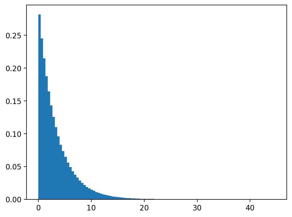
\[\begin{split} \begin{aligned} U& =F(X)=1-e^{-\lambda X}\qquad\\ \implies & \quad -U=e^{-\lambda X}\\ \implies& \quad \log(1-U)=-\lambda X\\ \implies & \quad X=\frac{(1-U)}{-\lambda} \end{aligned} \end{split}\]

Let’s draw \(u\) from \(U[0,1]\) and calculate \(x=\frac{log(1-U)}{-\lambda}\).

We’ll check whether \(X\) seems to follow a continuous geometric (exponential) distribution.

Let’s check with numpy.

n, λ = 1_000_000, 0.3

# draw uniform numbers
u = np.random.rand(n)

# transform
x = -np.log(1-u)/λ

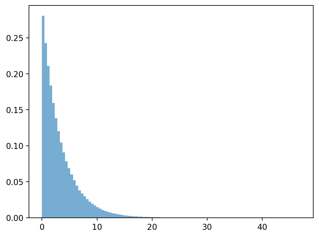
# draw geometric distributions
x_g = np.random.exponential(1 / λ, n)

# plot and compare
plt.hist(x, bins=100, density=True)
plt.show()

_images/ae0336cb6218b356b41308a6ab25cefb74418333ef779953eeac2f4f916cc7eb.png

plt.hist(x_g, bins=100, density=True, alpha=0.6)
plt.show()

_images/6e48458514b1f92dc56daa4affca215dc6d0480e80281dbf917d2cae8eab4a8c.png

Geometric distribution

Let \(X\) distributed geometrically, that is

\[\begin{split} \begin{aligned} \textrm{Prob}(X=i) & =(1-\lambda)\lambda^i,\quad\lambda\in(0,1), \quad i=0,1,\dots \\ & \sum_{i=0}^{\infty}\textrm{Prob}(X=i)=1\longleftrightarrow(1- \lambda)\sum_{i=0}^{\infty}\lambda^i=\frac{1-\lambda}{1-\lambda}=1 \end{aligned} \end{split}\]

Its CDF is given by

\[\begin{split} \begin{aligned} \textrm{Prob}(X\le i)& =(1-\lambda)\sum_{j=0}^{i}\lambda^i\\ & =(1-\lambda)[\frac{1-\lambda^{i+1}}{1-\lambda}]\\ & =1-\lambda^{i+1}\\ & =F(X)=F_i \quad \end{aligned} \end{split}\]

Again, let \(\tilde{U}\) follow a uniform distribution and we want to find \(X\) such that \(F(X)=\tilde{U}\).

Let’s deduce the distribution of \(X\) from

\[\begin{split} \begin{aligned} \tilde{U} & =F(X)=1-\lambda^{x+1}\\ 1-\tilde{U} & =\lambda^{x+1}\\ \log(1-\tilde{U})& =(x+1)\log\lambda\\ \frac{\log(1-\tilde{U})}{\log\lambda}& =x+1\\ \frac{\log(1-\tilde{U})}{\log\lambda}-1 &=x \end{aligned} \end{split}\]

However, \(\tilde{U}=F^{-1}(X)\) may not be an integer for any \(x\geq0\).

So let

\[ x=\lceil\frac{\log(1-\tilde{U})}{\log\lambda}-1\rceil \]

where \(\lceil . \rceil\) is the ceiling function.

Thus \(x\) is the smallest integer such that the discrete geometric CDF is greater than or equal to \(\tilde{U}\).

We can verify that \(x\) is indeed geometrically distributed by the following numpy program.

Note

The exponential distribution is the continuous analog of geometric distribution.

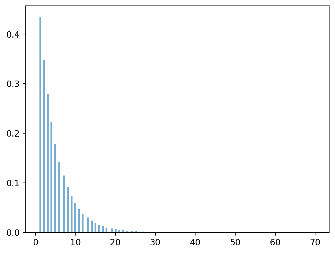
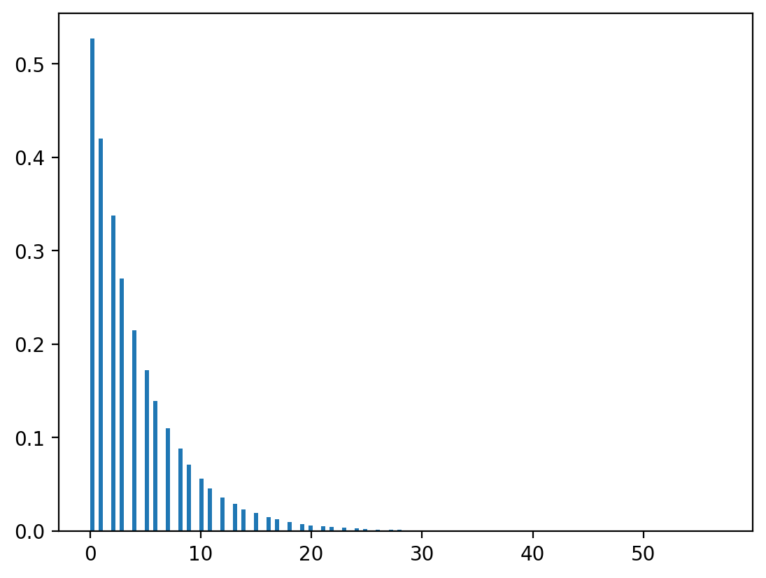
n, λ = 1_000_000, 0.8

# draw uniform numbers
u = np.random.rand(n)

# transform
x = np.ceil(np.log(1-u)/np.log(λ) - 1)

# draw geometric distributions
x_g = np.random.geometric(1-λ, n)

# plot and compare
plt.hist(x, bins=150, density=True)
plt.show()

_images/a582b3c99dea9e81a9126553140bb941473578976e2463cd31af72c73c674711.png

np.random.geometric(1-λ, n).max()

np.log(0.4)/np.log(0.3)

0.7610560044063084

plt.hist(x_g, bins=150, density=True, alpha=0.6)
plt.show()

_images/9ff3c40c69ce0d22f778affba7d4bfba20c5b8afbce9520e8bde8c1393a1eab7.png