65. Optimal Savings V: The Endogenous Grid Method#
In addition to what’s in Anaconda, this lecture will need the following libraries:
!pip install quantecon
65.1. Overview#
Previously, we solved the optimal savings problem using
We found time iteration to be significantly more accurate and efficient.
In this lecture, we’ll look at a clever twist on time iteration called the endogenous grid method (EGM).
EGM is a numerical method for implementing policy iteration invented by Chris Carroll.
The original reference is [Carroll, 2006].
For now we will focus on a clean and simple implementation of EGM that stays close to the underlying mathematics.
Then, in Optimal Savings VI: EGM with JAX, we will construct a fully vectorized and parallelized version of EGM based on JAX.
Let’s start with some standard imports:
import matplotlib.pyplot as plt
import numpy as np
import quantecon as qe
65.2. Key Idea#
First we remind ourselves of the theory and then we turn to numerical methods.
65.2.1. Theory#
We work with the model set out in Optimal Savings IV: Time Iteration, following the same terminology and notation.
As we saw, the Coleman-Reffett operator is a nonlinear operator \(K\) engineered so that the optimal policy \(\sigma^*\) is a fixed point of \(K\).
It takes as its argument a continuous strictly increasing consumption policy \(\sigma \in \Sigma\).
It returns a new function \(K \sigma\), where \((K \sigma)(x)\) is the \(c \in (0, \infty)\) that solves
65.2.2. Exogenous Grid#
As discussed in Optimal Savings IV: Time Iteration, to implement the method on a computer, we represent a policy function by a set of values on a finite grid.
The function itself is reconstructed from this representation when necessary, using interpolation or some other method.
Our previous strategy in Optimal Savings IV: Time Iteration for obtaining a finite representation of an updated consumption policy was to
fix a grid of income points \(\{x_i\}\)
calculate the consumption value \(c_i\) corresponding to each \(x_i\) using (65.1) and a root-finding routine
Each \(c_i\) is then interpreted as the value of the function \(K \sigma\) at \(x_i\).
Thus, with the pairs \(\{(x_i, c_i)\}\) in hand, we can reconstruct \(K \sigma\) via approximation.
Iteration then continues…
65.2.3. Endogenous Grid#
The method discussed above requires a root-finding routine to find the \(c_i\) corresponding to a given income value \(x_i\).
Root-finding is costly because it typically involves a significant number of function evaluations.
As pointed out by Carroll [Carroll, 2006], we can avoid this step if \(x_i\) is chosen endogenously.
The only assumption required is that \(u'\) is invertible on \((0, \infty)\).
Let \((u')^{-1}\) be the inverse function of \(u'\).
The idea is this:
First, we fix an exogenous grid \(\{s_i\}\) for savings (\(s = x - c\)).
Then we obtain \(c_i\) via
Finally, for each \(c_i\) we set \(x_i = c_i + s_i\).
Importantly, each \((x_i, c_i)\) pair constructed in this manner satisfies (65.1).
With the points \(\{x_i, c_i\}\) in hand, we can reconstruct \(K \sigma\) via approximation as before.
The name EGM comes from the fact that the grid \(\{x_i\}\) is determined endogenously.
65.3. Implementation#
As in Optimal Savings IV: Time Iteration, we will start with a simple setting where
\(u(c) = \ln c\),
the function \(f\) has a Cobb-Douglas specification, and
the shocks are lognormal.
This will allow us to make comparisons with the analytical solutions.
def v_star(x, α, β, μ):
    """
    True value function
    """
    c1 = np.log(1 - α * β) / (1 - β)
    c2 = (μ + α * np.log(α * β)) / (1 - α)
    c3 = 1 / (1 - β)
    c4 = 1 / (1 - α * β)
    return c1 + c2 * (c3 - c4) + c4 * np.log(x)

def σ_star(x, α, β):
    """
    True optimal policy
    """
    return (1 - α * β) * x
We reuse the Model structure from Optimal Savings IV: Time Iteration.
from typing import NamedTuple, Callable

class Model(NamedTuple):
    u: Callable           # utility function
    f: Callable           # production function
    β: float              # discount factor
    μ: float              # shock location parameter
    ν: float              # shock scale parameter
    s_grid: np.ndarray    # exogenous savings grid
    shocks: np.ndarray    # shock draws
    α: float              # production function parameter
    u_prime: Callable     # derivative of utility
    f_prime: Callable     # derivative of production
    u_prime_inv: Callable # inverse of u_prime


def create_model(
        u: Callable,
        f: Callable,
        β: float = 0.96,
        μ: float = 0.0,
        ν: float = 0.1,
        grid_max: float = 4.0,
        grid_size: int = 120,
        shock_size: int = 250,
        seed: int = 1234,
        α: float = 0.4,
        u_prime: Callable = None,
        f_prime: Callable = None,
        u_prime_inv: Callable = None
    ) -> Model:
    """
    Creates an instance of the optimal savings model.
    """
    # Set up exogenous savings grid
    s_grid = np.linspace(1e-4, grid_max, grid_size)

    # Store shocks (with a seed, so results are reproducible)
    np.random.seed(seed)
    shocks = np.exp(μ + ν * np.random.randn(shock_size))

    return Model(
        u, f, β, μ, ν, s_grid, shocks, α, u_prime, f_prime, u_prime_inv
    )
65.3.1. The Operator#
Here’s an implementation of \(K\) using EGM as described above.
def K(
        c_in: np.ndarray,   # Consumption values on the endogenous grid
        x_in: np.ndarray,   # Current endogenous grid
        model: Model        # Model specification
    ):
    """
    An implementation of the Coleman-Reffett operator using EGM.

    """

    # Simplify names
    u, f, β, μ, ν, s_grid, shocks, α, u_prime, f_prime, u_prime_inv = model

    # Linear interpolation of policy on the endogenous grid
    σ = lambda x: np.interp(x, x_in, c_in)

    # Allocate memory for new consumption array
    c_out = np.empty_like(s_grid)

    for i, s in enumerate(s_grid):
        # Approximate marginal utility ∫ u'(σ(f(s, α)z)) f'(s, α) z ϕ(z)dz
        vals = u_prime(σ(f(s, α) * shocks)) * f_prime(s, α) * shocks
        mu = np.mean(vals)
        # Compute consumption
        c_out[i] = u_prime_inv(β * mu)

    # Determine corresponding endogenous grid
    x_out = s_grid + c_out        # x_i = s_i + c_i

    return c_out, x_out
Note the lack of any root-finding algorithm.
Note
The routine is still not particularly fast because we are using pure Python loops.
But in the next lecture (Optimal Savings VI: EGM with JAX) we will use a fully vectorized and efficient solution.
65.3.2. Testing#
First we create an instance.
# Define utility and production functions with derivatives
u = lambda c: np.log(c)
u_prime = lambda c: 1 / c
u_prime_inv = lambda x: 1 / x
f = lambda k, α: k**α
f_prime = lambda k, α: α * k**(α - 1)

model = create_model(u=u, f=f, u_prime=u_prime,
                     f_prime=f_prime, u_prime_inv=u_prime_inv)
s_grid = model.s_grid
Here’s our solver routine:
def solve_model_time_iter(
        model: Model,             # Model details
        c_init: np.ndarray,       # initial guess of consumption on EG
        x_init: np.ndarray,       # initial guess of endogenous grid
        tol: float = 1e-5,        # Error tolerance
        max_iter: int = 1000,     # Max number of iterations of K
        verbose: bool = True      # If true print output
    ):
    """
    Solve the model using time iteration with EGM.
    """
    c, x = c_init, x_init
    error = tol + 1
    i = 0

    while error > tol and i < max_iter:
        c_new, x_new = K(c, x, model)
        error = np.max(np.abs(c_new - c))
        c, x = c_new, x_new
        i += 1
        if verbose:
            print(f"Iteration {i}, error = {error}")

    if i == max_iter:
        print("Warning: maximum iterations reached")

    return c, x
Let’s call it:
c_init = np.copy(s_grid)
x_init = s_grid + c_init
c, x = solve_model_time_iter(model, c_init, x_init)
Iteration 1, error = 1.208333333333333
Iteration 2, error = 0.6834464555052788
Iteration 3, error = 0.3126351338414741
Iteration 4, error = 0.12905177785629984
Iteration 5, error = 0.05099394329538409
Iteration 6, error = 0.01980055511172729
Iteration 7, error = 0.007636088144566955
Iteration 8, error = 0.002937098891578671
Iteration 9, error = 0.0011285611196765188
Iteration 10, error = 0.00043347299641638415
Iteration 11, error = 0.00016646919532892213
Iteration 12, error = 6.392646634978405e-05
Iteration 13, error = 2.4548101555943447e-05
Iteration 14, error = 9.426520908739633e-06
Here is a plot of the resulting policy, compared with the true policy:
fig, ax = plt.subplots()

ax.plot(x, c, lw=2,
        alpha=0.8, label='approximate policy function')

ax.plot(x, σ_star(x, model.α, model.β), 'k--',
        lw=2, alpha=0.8, label='true policy function')

ax.legend()
plt.show()
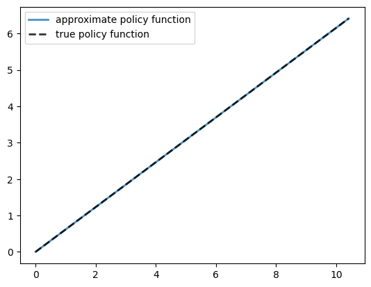
The maximal absolute deviation between the two policies is
np.max(np.abs(c - σ_star(x, model.α, model.β)))
np.float64(2.2564941266622895e-06)
Here’s the execution time:
with qe.Timer():
    c, x = solve_model_time_iter(model, c_init, x_init, verbose=False)
0.0302 seconds elapsed
EGM is faster than time iteration because it avoids numerical root-finding.
Instead, we invert the marginal utility function directly, which is much more efficient.
In Optimal Savings VI: EGM with JAX, we will use a fully vectorized and efficient version of EGM that is also parallelized using JAX.
This provides an extremely fast way to solve the optimal consumption problem we have been studying for the last few lectures.