106. Econometric Policy Evaluation#
106.1. Overview#
This lecture follows chapter 9 of Sargent [1999], “Econometric Policy Evaluation”.
The preceding lectures built the adaptive governments of the book’s chapter 8 and studied them by simulation (Adaptive Learning and Escape Dynamics, Escaping Nash Inflation, Priors, Escapes, and Learning Cycles).
Chapter 9 takes the same models to U.S. data, estimating them by maximum likelihood under both the classical and the Keynesian identification schemes, following Chung [1990].
It is the book’s only structural confrontation of the vindication story of The Rise and Fall of U.S. Inflation with data.
The question is counterfactual: what would a policy adviser of the 1960s and 1970s have recommended if he had fit a distributed-lag Phillips curve, discounted old data, and fed the estimates into the Phelps problem of Adaptive Expectations and the Phelps Problem?
The estimated model answers directly, because in it the fitted value of inflation is the government’s recommendation.
Once the gain and the discount factor are fixed, the likelihood has no free parameters describing beliefs: we compute the government’s beliefs and recommendations from the data, as the government itself would have.
We reproduce the book’s main findings:
both models fit inflation badly, and the classical model fits much worse;
the misses are systematic, with recommended inflation below actual inflation through the 1970s, which is the sense in which “the pattern of misses from the estimated models favors vindication”;
the Keynesian government’s estimated Phillips curve satisfied the induction hypothesis by the mid-1970s, and its plans called for low inflation years before Volcker arrived;
the classical government recommended low inflation all along, which is why its recommendations “would have been even more timely.”
The book does not report its lag lengths or how it converted its data to quarterly frequency, and we say where these choices matter.
Let’s start with some imports.
import matplotlib.pyplot as plt
import numpy as np
import pandas as pd
from scipy.linalg import solve_discrete_are
from scipy.optimize import minimize
from scipy.signal import lfilter
from scipy.stats import chi2
106.2. The model#
The model combines the actual Phillips curve of Self-Confirming Equilibria with the adaptive government of Adaptive Learning and Escape Dynamics; the notation is that of A note on notation.
106.2.1. The actual Phillips curve#
With \(U_t\) unemployment, \(y_t\) inflation and \(x_t\) the public’s expectation of inflation, the economy obeys a natural-rate Phillips curve with a geometric distributed lag in surprise inflation \(v_{2t} = y_t - x_t\) and a serially correlated disturbance:
where \(L\) is the lag operator, \(|\rho_1| < 1\) and \(|\rho_2| < 1\).
Multiplying through by \((1-\rho_1 L)(1-\rho_2 L)\) gives the form that the book numbers (48):
The shock vector \(v_t = (v_{1t}, v_{2t})^\top\) is Gaussian white noise with an unrestricted covariance matrix \(V_v\).
Chapters 7 and 8 of the book set \(\rho_1 = \rho_2 = 0\) and made \(V_v\) diagonal to make theoretical points; chapter 9 frees both.
106.2.2. The government#
Let \(X_{t-1} = \begin{bmatrix} U_{t-1} & \cdots & U_{t-m_U} & y_{t-1} & \cdots & y_{t-m_y} & 1 \end{bmatrix}^\top\) collect information dated \(t-1\) and earlier.
As in Adaptive Expectations and the Phelps Problem, the government fits one of two reduced-form Phillips curves, which differ only in their direction of fit:
where \(X_{C,t} = \begin{bmatrix} y_t & X_{t-1}^\top \end{bmatrix}^\top\) and \(X_{K,t} = \begin{bmatrix} U_t & X_{t-1}^\top \end{bmatrix}^\top\).
It re-estimates its curve every period by constant-gain recursive least squares, which for the classical scheme is
with a constant gain \(g = 1 - \lambda\); the Keynesian scheme updates \(\beta_t\) and \(R_{XK,t}\) in the same way.
A Keynesian government converts its estimate into the classical form by inverting the Phillips curve: if \(\beta_1\) is the coefficient on \(U_t\) and \(\beta_{-1}\) collects the rest, then \(\gamma(\beta) = \begin{bmatrix} \beta_1^{-1} & -\beta_{-1}^\top/\beta_1 \end{bmatrix}^\top\).
Each period the government acts as if its current estimate will govern the Phillips curve forever and sets inflation by solving the Phelps problem, minimizing \(\mathbb{E}\sum_t \delta^t (U_t^2 + y_t^2)\) subject to its estimated curve, which yields the rule
where \(\gamma_{t-1}\) is the classical estimate or \(\gamma(\beta_{t-1})\), and \(v_{2t}\) is a control error.
Following Sims [1988] and Chung [1990], the public knows the rule, so \(x_t = h(\gamma_{t-1}) X_{t-1}\), and the control error \(v_{2t}\) is also the inflation surprise in (106.1).
106.3. The likelihood function#
To simulate the model, we would draw shocks \(\{v_t\}\) and compute histories of \((y_t, U_t)\) and of the government’s beliefs.
To estimate it, we reverse the procedure: starting from initial beliefs, we use the data \(\{y_t, U_t\}\) to solve for the shocks that would have produced them,
while updating \(\gamma_t\) (or \(\beta_t\)) by (106.4); these are the book’s equations (105).
Given the past, the map from \(v_t\) to \((U_t, y_t)\) is triangular with unit diagonal, so its Jacobian is one and the Gaussian log likelihood of a sample of length \(T\) is
As the book suggests, we concentrate out \(V_v\): its maximizer is \(\hat V_v = T^{-1}\sum_t v_t v_t^\top\), and then \(\log L = -T\log 2\pi - \frac{T}{2}\log\det \hat V_v - T\).
Note
The book’s appendix to chapter 9 writes the log of a sum of densities where it means a sum of log densities, and gives the constant as \(-\frac{T}{2}\log 2\pi\), which is right for a scalar observation; a bivariate density has \(-T\log 2\pi\).
Neither misprint affects the estimates, but the second shifts the level of \(\log L\).
The book estimates \((\theta, U^*, \rho_1, \rho_2, V_v)\), and it fixes the discount factor at \(\delta = .999\) and the forgetting factor at \(\lambda = .985\), so the gain is \(g = .015\).
Notice what is not on the list: nothing describes beliefs.
With \(\lambda\), \(\delta\) and the initial beliefs fixed, the government’s beliefs \(\gamma_t\), its recommendations \(h(\gamma_{t-1})X_{t-1}\) and therefore its misses \(v_{2t}\) are computed from the data alone, whatever the values of the parameters being estimated.
This has two consequences.
Because \(\det \hat V_v\) equals the mean square of \(v_{2t}\) times the mean square of the part of \(v_{1t}\) not explained by \(v_{2t}\), the parameters \((\theta, U^*, \rho_1, \rho_2)\) are estimated from the unemployment equation, taking the government’s misses as given.
The comparison between the two identification schemes is mostly a comparison of the size of their misses, that is, of how far the recommendations were from what actually happened.
This is a cross-equation restriction of the kind familiar from rational expectations econometrics: the government’s rule is pinned down by its econometrics and the Phelps problem, not left free.
106.4. Data#
Chapter 9 uses the measures of chapter 1: the consumer price index (all items) and the unemployment rate of white men aged 20 and over, the series plotted in The Rise and Fall of U.S. Inflation.
Although chapter 1 plots monthly data, chapter 9’s estimates appear to be quarterly:
the sample period is dated in quarters (it is printed as “1995I–1997I”, evidently a misprint for 1955I–1997I, since the figures begin in 1955);
Figure 9.2b refers to “the first quarter of 1960”;
quarterly data reproduce the book’s estimates and figures closely, while monthly data do not, for a reason we explain below.
We therefore convert the monthly series to quarterly by taking the last month of each quarter, and measure inflation as the annualized percentage change in the CPI.
Because we sample one month per quarter, we use the seasonally adjusted index rather than the unadjusted one plotted in The Rise and Fall of U.S. Inflation.
def read_fred(series_id):
    "Read a monthly series from FRED."
    url = f'https://fred.stlouisfed.org/graph/fredgraph.csv?id={series_id}'
    s = pd.read_csv(url, index_col=0, parse_dates=True)[series_id]
    return pd.to_numeric(s, errors='coerce')

cpi_monthly = read_fred('CPIAUCSL')     # CPI, all items, seasonally adjusted
u_monthly = read_fred('LNS14000028')    # unemployment rate, white men 20+

def make_data(how='last', end='1997-03'):
    "Inflation (annualized percent) and unemployment at quarterly or monthly frequency."
    if how == 'monthly':
        cpi, u, scale = cpi_monthly, u_monthly, 1200
    elif how == 'last':                         # last month of each quarter
        cpi, u, scale = (cpi_monthly.resample('QS').last(),
                         u_monthly.resample('QS').last(), 400)
    else:                                       # quarterly averages
        cpi, u, scale = (cpi_monthly.resample('QS').mean(),
                         u_monthly.resample('QS').mean(), 400)
    y = scale * np.log(cpi).diff()
    data = pd.concat([y.rename('y'), u.rename('U')], axis=1).dropna()
    return data.loc[:end]

data = make_data()
print(f"{data.index[0]:%Y-%m} to {data.index[-1]:%Y-%m}: {len(data)} quarters")
1954-01 to 1997-01: 173 quarters
The unemployment series begins in 1954, and the government’s regression needs a few years of data before its estimates mean anything.
So we treat 1954–1957 as a training sample for the government’s beliefs and evaluate the likelihood from 1958Q1 through 1997Q1.
The book does not report its lag lengths \(m_U\) and \(m_y\); the simulations of its chapter 8 used two lags of each.
We use one lag of unemployment and two of inflation, which among the lag lengths we tried puts our estimates closest to the book’s; the robustness table below shows what changes with two lags of each.
106.5. Beliefs and recommendations#
The Phelps problem is the discounted LQ problem of Adaptive Learning and Escape Dynamics, generalized to any number of lags.
Write the believed Phillips curve as \(U_t = \gamma_0 y_t + c^\top s_t\) with state \(s_t = X_{t-1}\), so that the per-period loss is \(s_t^\top c c^\top s_t + (\gamma_0^2 + 1) y_t^2 + 2 \gamma_0 y_t c^\top s_t\).
We use the same solver as Adaptive Learning and Escape Dynamics: in the discounted problem only \(A\) and \(B\) are multiplied by \(\sqrt{\delta}\), and the cross term \(N\) is passed to the Riccati solver unscaled.
def lq_matrices(γ, mU, my):
    """
    Believed law of motion s_{t+1} = A s_t + B y_t for the state
    s_t = [U_{t-1},...,U_{t-mU}, y_{t-1},...,y_{t-my}, 1]
    when the believed Phillips curve is U_t = γ[0] y_t + γ[1:] @ s_t.
    """
    γ0, c = γ[0], γ[1:]
    n = mU + my + 1
    A, B = np.zeros((n, n)), np.zeros((n, 1))
    if mU > 0:
        A[0, :], B[0, 0] = c, γ0                 # U_t
        for j in range(1, mU):
            A[j, j - 1] = 1.0
    if my > 0:
        B[mU, 0] = 1.0                           # y_t
        for j in range(mU + 1, mU + my):
            A[j, j - 1] = 1.0
    A[-1, -1] = 1.0                              # constant
    return A, B

def phelps_h(γ, δ, mU, my):
    "Phelps rule y_t = h @ s_t for the believed Phillips curve γ."
    γ0, c = γ[0], γ[1:]
    A, B = lq_matrices(γ, mU, my)
    R = np.outer(c, c)
    Q = np.array([[γ0**2 + 1.0]])
    N = (γ0 * c).reshape(1, -1)
    Ad, Bd = np.sqrt(δ) * A, np.sqrt(δ) * B
    P = solve_discrete_are(Ad, Bd, R, Q, s=N.T)
    F = np.linalg.solve(Q + Bd.T @ P @ Bd, Bd.T @ P @ Ad + N)
    return -F.ravel()

def γ_of_β(β):
    "Invert a Keynesian Phillips curve into classical form."
    return np.concatenate([[1 / β[0]], -β[1:] / β[0]])
With a diffuse initial condition, \(R_{XC,-1} = 0\), the recursion (106.4) delivers discounted least squares: \(\gamma_t\) minimizes \(\sum_{s \le t} \lambda^{t-s} (U_s - \gamma^\top X_{C,s})^2\), so an observation \(k\) quarters old gets weight \(\lambda^k\).
The function below computes the beliefs this way from the first quarter of data, and rebuilds, quarter by quarter, the recommendation \(h(\gamma_{t-1}) X_{t-1}\) that the government would have made.
def government(data, scheme, λ=0.985, δ=0.999, mU=1, my=2, n_init=8):
    """
    Beliefs and recommendations of a government that fits the classical ('C')
    or Keynesian ('K') Phillips curve by discounted least squares and solves
    the Phelps problem, reconstructed from data on (y, U).
    """
    U, y = data['U'].to_numpy(), data['y'].to_numpy()
    T, k, m = len(U), mU + my + 2, max(mU, my)
    S, b, zz, w = np.zeros((k, k)), np.zeros(k), 0.0, 0.0
    coef = np.full((T, k), np.nan)
    S_path, σ2 = np.full((T, k, k), np.nan), np.full(T, np.nan)
    states, yhat = np.full((T, k - 1), np.nan), np.full(T, np.nan)
    for t in range(m, T):
        s = np.concatenate([U[t - mU:t][::-1], y[t - my:t][::-1], [1.0]])
        states[t] = s
        if t - m > n_init:                       # recommendation from γ_{t-1}
            β = coef[t - 1]
            γ = β if scheme == 'C' else γ_of_β(β)
            yhat[t] = phelps_h(γ, δ, mU, my) @ s
        x = np.r_[y[t], s] if scheme == 'C' else np.r_[U[t], s]
        z = U[t] if scheme == 'C' else y[t]
        S, b = λ * S + np.outer(x, x), λ * b + x * z
        zz, w = λ * zz + z**2, λ * w + 1
        if t - m >= n_init:
            coef[t] = np.linalg.solve(S, b)
            S_path[t] = S
            σ2[t] = (zz - b @ coef[t]) / (w - k)  # discounted residual variance
    lags_y = coef[:, 1 + mU:1 + mU + my].sum(axis=1)
    out = data.copy()
    out['yhat'] = yhat
    out['miss'] = out['y'] - out['yhat']           # v_2t
    out['sum_y'] = lags_y + coef[:, 0] if scheme == 'C' else lags_y
    return dict(frame=out, coef=coef, S=S_path, σ2=σ2, states=states,
                scheme=scheme, λ=λ, δ=δ, mU=mU, my=my)

gov = {s: government(data, s) for s in 'CK'}
106.6. Estimates#
The function loglik evaluates (106.7) with \(V_v\) concentrated out.
It uses data from two quarters before the likelihood sample to supply \(U_{t-1}\) and \(U_{t-2}\), and, as the book does, it sets the pre-sample shocks to zero.
def residuals(params, U, v2):
    "Solve the actual Phillips curve for v_1 given the misses v_2."
    θ, U_star, ρ1, ρ2 = params
    U0, U1, U2 = U[2:], U[1:-1], U[:-2]
    v2 = v2[2:]
    v2_lag = np.r_[0.0, v2[:-1]]
    rhs = (θ * (v2 - ρ1 * v2_lag) + U0 - (ρ1 + ρ2) * U1 + ρ1 * ρ2 * U2
           - U_star * (1 - ρ1) * (1 - ρ2))
    v1 = lfilter([1.0], [1.0, -ρ2], rhs)           # v1_t = ρ2 v1_{t-1} + rhs_t
    return v1, v2

def loglik(params, U, v2):
    "Gaussian log likelihood with V_v concentrated out."
    v = np.vstack(residuals(params, U, v2))
    T = v.shape[1]
    V = v @ v.T / T
    return -T * np.log(2 * np.pi) - T / 2 * np.linalg.slogdet(V)[1] - T, V

def estimate(g, start='1958'):
    "Maximum likelihood estimates of (θ, U*, ρ1, ρ2) for a government g."
    f = g['frame']
    i0 = f.index.get_loc(pd.Timestamp(start)) - 2
    U, v2 = f['U'].to_numpy()[i0:], f['miss'].to_numpy()[i0:]

    def neg(p):
        return -loglik(p, U, v2)[0] if max(abs(p[2]), abs(p[3])) < 1 else 1e10

    starts = [(0.2, 4.0, ρ1, ρ2) for ρ1 in (0.8, 0.95) for ρ2 in (0.0, 0.5, 0.9)]
    fits = [minimize(neg, x0, method='Nelder-Mead',
                     options=dict(xatol=1e-8, fatol=1e-9, maxiter=20_000))
            for x0 in starts]
    best = min(fits, key=lambda r: r.fun)
    return dict(params=best.x, loglik=-best.fun, U=U, v2=v2,
                V=loglik(best.x, U, v2)[1], T=len(U) - 2)

def std_errors(est, h=1e-4):
    "Standard errors from the numerical Hessian of the concentrated likelihood."
    x, k = est['params'], len(est['params'])
    f = lambda p: loglik(p, est['U'], est['v2'])[0]
    E, H = h * np.eye(k), np.empty((k, k))
    for i in range(k):
        for j in range(k):
            H[i, j] = (f(x + E[i] + E[j]) - f(x + E[i] - E[j])
                       - f(x - E[i] + E[j]) + f(x - E[i] - E[j])) / (4 * h**2)
    return np.sqrt(np.diag(np.linalg.inv(-H)))

est = {s: estimate(gov[s]) for s in 'CK'}
se = {s: std_errors(est[s]) for s in 'CK'}
Here are our estimates next to the book’s Tables 3 and 4.
book = {'C': [0.1192, 1.6483, 0.9145, 0.5754, -560],
        'K': [0.163, 2.745, 0.932, 0.667, -333]}
names = ['θ', 'U*', 'ρ1', 'ρ2']
rows = []
for s, label in [('C', 'classical'), ('K', 'Keynesian')]:
    for i, name in enumerate(names):
        p, e = est[s]['params'][i], se[s][i]
        rows.append([label, name, book[s][i], p, e, abs(p - book[s][i]) / e])
    rows.append([label, 'log L', book[s][4], est[s]['loglik'], np.nan, np.nan])
table = pd.DataFrame(rows, columns=['scheme', 'parameter', 'book', 'ours',
                                    'std. error', '|ours - book| / s.e.'])
print(f"likelihood sample: {est['C']['T']} quarters, 1958Q1-1997Q1")
table.set_index(['scheme', 'parameter']).round(3)
likelihood sample: 157 quarters, 1958Q1-1997Q1
| book | ours | std. error | |ours - book| / s.e. | ||
|---|---|---|---|---|---|
| scheme | parameter | ||||
| classical | θ | 0.119 | 0.115 | 0.042 | 0.097 |
| U* | 1.648 | 0.424 | 1.158 | 1.057 | |
| ρ1 | 0.914 | 0.915 | 0.025 | 0.034 | |
| ρ2 | 0.575 | 0.695 | 0.081 | 1.480 | |
| log L | -560.000 | -587.608 | NaN | NaN | |
| Keynesian | θ | 0.163 | 0.169 | 0.056 | 0.106 |
| U* | 2.745 | 2.786 | 0.604 | 0.069 | |
| ρ1 | 0.932 | 0.922 | 0.026 | 0.403 | |
| ρ2 | 0.667 | 0.720 | 0.071 | 0.745 | |
| log L | -333.000 | -457.271 | NaN | NaN |
The book’s estimates of \(\theta\) and \(\rho_1\) lie within a fraction of a standard error of ours under both schemes; its values of \(U^*\) and \(\rho_2\) are within about one and a half of our standard errors.
The impact effect \(\theta\) of an inflation surprise is small, between a tenth and a fifth of a percentage point of unemployment per percentage point of annualized quarterly inflation.
The Phillips-curve disturbance is persistent (\(\rho_1\) above .9), and the effect of a surprise decays faster (\(\rho_2\) near .7).
Two parameters are weakly determined: the estimate of \(\rho_2\) moves noticeably if the likelihood sample starts two quarters later, after the 1958 recession,
for s, label in [('C', 'classical'), ('K', 'Keynesian')]:
    p = estimate(gov[s], start='1958-07')['params']
    print(f"{label:10s} from 1958Q3: θ = {p[0]:.3f}, U* = {p[1]:.2f}, "
          f"ρ1 = {p[2]:.3f}, ρ2 = {p[3]:.3f}")
classical  from 1958Q3: θ = 0.114, U* = 0.34, ρ1 = 0.924, ρ2 = 0.519
Keynesian  from 1958Q3: θ = 0.138, U* = 2.60, ρ1 = 0.938, ρ2 = 0.612
and the natural rate \(U^*\) has a large standard error.
The Keynesian scheme has a much higher likelihood.
Our gap between the two schemes is smaller than the book’s; the levels of \(\log L\) are not comparable, because of the misprinted constant and different data vintages, but the sign of the gap is the same.
The residuals show where the gap comes from, and why \(U^*\) is hard to pin down:
for s, label in [('C', 'classical'), ('K', 'Keynesian')]:
    v1, v2 = residuals(est[s]['params'], est[s]['U'], est[s]['v2'])
    rms = lambda v: np.sqrt(np.mean(v**2))
    print(f"{label:10s}: misses v2: root mean square {rms(v2):.2f}, mean {v2.mean():.2f};  "
          f"v1: root mean square {rms(v1):.2f}, mean {v1.mean():.2f};  "
          f"corr(v1, v2) = {np.corrcoef(v1, v2)[0, 1]:.2f}")
print(f"average unemployment over the sample: {est['C']['U'][2:].mean():.2f}")
classical : misses v2: root mean square 6.82, mean 6.08;  v1: root mean square 0.69, mean 0.52;  corr(v1, v2) = 0.58
Keynesian : misses v2: root mean square 3.11, mean 1.55;  v1: root mean square 0.51, mean 0.19;  corr(v1, v2) = 0.68
average unemployment over the sample: 4.44
The classical government’s misses are more than twice as large, in root mean square, as the Keynesian government’s.
Both sets of misses have a positive mean, because the recommendations lay below actual inflation for long stretches.
Because \(v_1\) is correlated with \(v_2\), it can have a positive mean too, and a low \(U^*\) combined with a positive mean of \(v_1\) fits nearly as well as a higher \(U^*\); that is presumably why both the book and we find values of \(U^*\) below the average unemployment rate.
106.7. Recommendations and misses#
The fitted value of inflation in this model is not a forecast made by an outside econometrician: it is the inflation rate that the government’s own procedure recommended, given the data it had seen.
The next two figures reproduce the book’s Figures 9.1 and 9.2a: each shows the recommendation against actual inflation, and the sum of the coefficients on inflation in the government’s estimated Phillips curve.
The induction hypothesis (Testing the natural-rate hypothesis) holds when that sum is \(0\) in the classical regression and \(1\) in the Keynesian regression.
def plot_government(g, ref, title, sum_label, start='1958'):
    f = g['frame'].loc[start:]
    fig, axes = plt.subplots(2, 1, figsize=(9, 7), sharex=True)
    axes[0].plot(f.index, f['y'], 'C0--', lw=1, label='actual')
    axes[0].plot(f.index, f['yhat'], 'C1', lw=1.8, label='recommended')
    axes[0].axhline(0, color='k', lw=0.5)
    axes[0].set_ylabel('inflation (percent)')
    axes[0].legend(frameon=False)
    axes[1].plot(f.index, f['sum_y'], 'C2', lw=1.5)
    axes[1].axhline(ref, color='k', ls=':', lw=1, label='induction hypothesis')
    axes[1].set_ylabel(sum_label)
    axes[1].legend(frameon=False)
    axes[0].set_title(title)
    plt.tight_layout()
    plt.show()
First the classical government.
plot_government(gov['C'], 0, 'Classical identification',
                'sum on current and lagged $y$')
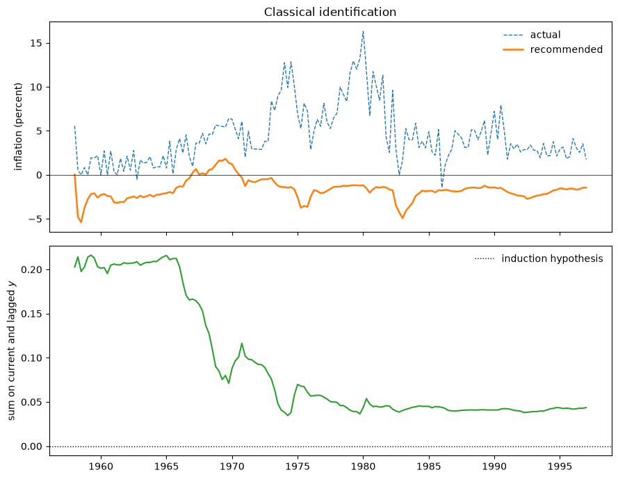
Fig. 106.1 Classical government: recommended and actual inflation, and the sum of coefficients on current and lagged inflation (book Figure 9.1)#
The classical government recommends inflation below zero almost throughout, rising above it only briefly around 1970.
As the book says, “the classical model fails even to match the acceleration in inflation leading up to 1970.”
Its regression of unemployment on current and lagged inflation finds coefficients on inflation whose sum is small, and close to zero from the early 1970s on.
Such a government sees almost no exploitable tradeoff, so the Phelps problem tells it to aim for low inflation.
plot_government(gov['K'], 1, 'Keynesian identification', 'sum on lagged $y$')
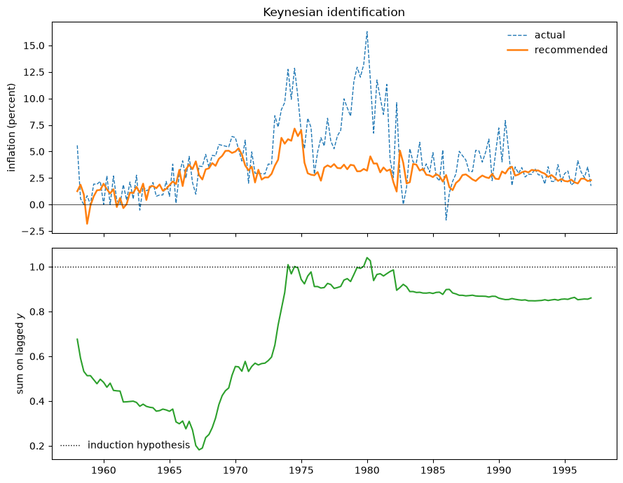
Fig. 106.2 Keynesian government: recommended and actual inflation, and the sum of coefficients on lagged inflation (book Figure 9.2a)#
The Keynesian recommendations reflect the inflation pattern better, partly matching the acceleration of the late 1960s.
From the early 1970s, however, they lie well below actual inflation, and they stay below it for most of the next two decades.
The lower panel shows why.
The sum of the weights on lagged inflation climbs from well below one in the 1960s to about one by the mid-1970s and stays near it.
By then the Keynesian government had learned the Solow–Tobin version of the natural-rate hypothesis, and the Phelps problem told it to bring inflation down.
106.7.1. The induction hypothesis emerges#
The book’s Figure 9.2b shows how the data gradually removed the government’s doubt.
We approximate the government’s uncertainty about \(\beta_t\) by \(\hat\sigma_t^2 \left(\sum_{s\le t}\lambda^{t-s} X_{K,s}X_{K,s}^\top\right)^{-1}\), with \(\hat\sigma_t^2\) the discounted residual variance.
This is the covariance matrix that a Kalman filter implementing constant-gain least squares would attach to its estimate.
The figure plots the 95 and 99 percent confidence ellipses for the sum of the weights on lagged inflation and the constant in the first quarter of 1960, 1965, …, 1985.
def ellipse(center, cov, level, n=200):
    "Points on a confidence ellipse for a bivariate normal estimate."
    w, Q = np.linalg.eigh(cov)
    a = np.linspace(0, 2 * np.pi, n)
    circle = np.vstack([np.cos(a), np.sin(a)])
    return center[:, None] + Q @ (np.sqrt(chi2.ppf(level, 2) * w)[:, None] * circle)

g = gov['K']
k = g['coef'].shape[1]
D = np.zeros((2, k))
D[0, 1 + g['mU']:1 + g['mU'] + g['my']] = 1.0     # sum of weights on lagged y
D[1, -1] = 1.0                                     # constant

fig, axes = plt.subplots(2, 3, figsize=(10, 6.5), sharex=True, sharey=True)
for ax, year in zip(axes.ravel(), range(1960, 1990, 5)):
    t = g['frame'].index.get_loc(pd.Timestamp(f'{year}-01-01'))
    center = D @ g['coef'][t]
    cov = g['σ2'][t] * D @ np.linalg.inv(g['S'][t]) @ D.T
    for level, ls in [(0.95, '-'), (0.99, '--')]:
        e = ellipse(center, cov, level)
        ax.plot(e[0], e[1], 'C0', ls=ls, lw=1)
    ax.plot(*center, 'C0o', ms=3)
    ax.axvline(1, color='k', ls=':', lw=1)
    ax.set_title(f'{year}Q1')
for ax in axes[1]:
    ax.set_xlabel('sum on lagged $y$')
for ax in axes[:, 0]:
    ax.set_ylabel('constant')
plt.tight_layout()
plt.show()
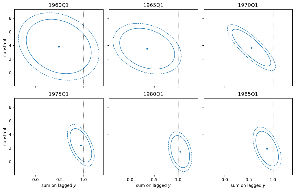
Fig. 106.3 Keynesian government: 95% and 99% confidence ellipses for the sum of weights on lagged inflation and the constant (book Figure 9.2b)#
The pattern resembles the book’s figure and the confidence ellipses from the simulations of its chapter 8.
In the 1960s the ellipses lie away from the induction hypothesis (the dotted line) but are large enough to leave room for doubt.
During the 1970s the centers move onto the induction hypothesis and stay there, and the ellipses become smaller than those of the early 1960s, though not as small as the book’s.
In the book’s words, the point estimates move, “causing the centers of the ellipsoids to shift and doubt to dwindle.”
106.8. Misses favor vindication#
Judged by period-by-period fit, the adaptive models are disappointing: there is a long string of under-predictions of inflation during the 1970s, even for the Keynesian model.
Sargent reads the misses differently:
But such misses do not necessarily fail to vindicate econometric policy evaluation. To the contrary, the pattern of misses from the estimated models favors vindication. Remembering that the fitted value from the adaptive model is the government’s recommendation as time passes extracts vindication from the econometric shortcomings.
The misses say that the recommendations were systematically lower than the inflation that actually occurred: the government’s procedure was telling it to disinflate while actual policy did not.
The one-step recommendation \(h(\gamma_{t-1})X_{t-1}\) mixes two things: where the government wanted inflation to go, and how fast it planned to get there from the inflation it inherited.
To separate them, we compute the steady state of the government’s plan, the long-run inflation rate toward which the Phelps rule would steer the economy if the current beliefs were correct.
def planned_long_run(γ, δ, mU, my):
    "Steady-state inflation of the government's plan under its own beliefs."
    h = phelps_h(γ, δ, mU, my)
    A, B = lq_matrices(γ, mU, my)
    M = A + B @ h[None, :]                         # believed closed loop
    n = M.shape[0] - 1                             # last state is the constant
    s_bar = np.linalg.solve(np.eye(n) - M[:n, :n], M[:n, -1])
    return h @ np.r_[s_bar, 1.0]

def long_run_path(g):
    path = np.full(len(g['frame']), np.nan)
    for t in range(1, len(path)):
        β = g['coef'][t - 1]
        if not np.isnan(β).any():
            γ = β if g['scheme'] == 'C' else γ_of_β(β)
            path[t] = planned_long_run(γ, g['δ'], g['mU'], g['my'])
    return pd.Series(path, index=g['frame'].index)

for s in 'CK':
    gov[s]['frame']['long_run'] = long_run_path(gov[s])
The next figure puts the Keynesian government’s plan next to its one-step recommendation, the classical recommendation, and actual inflation.
fK, fC = gov['K']['frame'].loc['1958':], gov['C']['frame'].loc['1958':]
fig, ax = plt.subplots(figsize=(9, 4.8))
ax.plot(fK.index, fK['y'], 'C0--', lw=1, label='actual inflation')
ax.plot(fK.index, fK['yhat'], 'C1', lw=1.5, label='Keynesian recommendation')
ax.plot(fK.index, fK['long_run'], 'C3', lw=2, label='Keynesian planned long-run inflation')
ax.plot(fC.index, fC['yhat'], 'C2', lw=1, alpha=0.8, label='classical recommendation')
ax.axvline(pd.Timestamp('1979-08-01'), color='k', ls=':', lw=1)
ax.text(pd.Timestamp('1980-06-01'), -4, 'Volcker', fontsize=9)
ax.axhline(0, color='k', lw=0.5)
ax.set_ylabel('percent')
ax.legend(frameon=False, fontsize=9, loc='upper left')
plt.show()
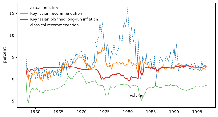
Fig. 106.4 Actual inflation, the Keynesian government’s recommendation, and the long-run inflation rate its plan aimed for#
Averages over five eras summarize the figure.
eras = [('1958', '1965'), ('1966', '1972'), ('1973', '1979'),
        ('1980', '1984'), ('1985', '1997')]
summary = pd.DataFrame(
    {f'{a}-{b}': [fK['y'].loc[a:b].mean(),
                  fC['yhat'].loc[a:b].mean(),
                  fK['yhat'].loc[a:b].mean(),
                  fK['long_run'].loc[a:b].median()]
     for a, b in eras},
    index=['actual inflation', 'classical recommendation',
           'Keynesian recommendation', 'Keynesian long-run plan (median)'])
summary.round(2)
| 1958-1965 | 1966-1972 | 1973-1979 | 1980-1984 | 1985-1997 | |
|---|---|---|---|---|---|
| actual inflation | 1.40 | 4.12 | 8.47 | 6.32 | 3.39 |
| classical recommendation | -2.56 | 0.08 | -1.72 | -2.36 | -1.82 |
| Keynesian recommendation | 1.18 | 3.60 | 4.14 | 3.23 | 2.60 |
| Keynesian long-run plan (median) | 2.62 | 2.41 | 0.80 | 0.74 | 2.71 |
From 1973 through 1990 the recommendations were mostly below actual inflation:
for s, label in [('C', 'classical'), ('K', 'Keynesian')]:
    m = gov[s]['frame']['miss'].loc['1973':'1990']
    print(f"{label:10s}: mean miss 1973-1990 = {m.mean():5.2f}, "
          f"share of quarters with recommendation below actual = {(m > 0).mean():.0%}")
classical : mean miss 1973-1990 =  8.26, share of quarters with recommendation below actual = 100%
Keynesian : mean miss 1973-1990 =  3.04, share of quarters with recommendation below actual = 86%
The computation bears out the book’s interpretation:
The econometric estimates tell us that unreconstructed Keynesian Phillips curve fitters would have detected the adverse shift in the empirical Phillips curve and through the induction hypothesis combined with the Phelps problem would have recommended lowering the inflation rate. Those quantitative policy evaluators would not have concurred with the loosely argued recommendations current in the late 1970’s that long lags in expectations made it too costly to disinflate. Our results say that recommendations under classical identification would have been even more timely.
Through the 1960s the Keynesian government aimed at a long-run inflation rate of two to three percent.
Once its estimated sum of weights on lagged inflation approached one, its target fell to about one percent or less, and it stayed there through the early 1980s, while actual inflation ran far higher.
Its one-step recommendations in the late 1970s, around four percent, called for cutting inflation well below the rates it inherited.
After the Volcker disinflation, the sum of weights drifted down a little and the planned long-run rate returned to two to three percent, close to actual inflation.
The classical government’s recommendations were close to zero even during the acceleration of the late 1960s, and below zero after it: that is the sense in which they “would have been even more timely.”
Chapter 1 of the book draws the moral: “The econometric estimates present the mystery of why the stabilization was postponed.”
106.8.1. How robust are the misses?#
Because the book does not report its lag lengths or its conversion to quarterly data, the table varies the lags, the quarterly sampling, and the frequency.
The monthly columns use \(\lambda^{1/3}\) and \(\delta^{1/3}\), which keep the same memory and the same discounting in calendar time.
specs = [('end of quarter', 'last', 1, 2), ('end of quarter', 'last', 2, 2),
         ('quarterly average', 'avg', 1, 2), ('quarterly average', 'avg', 2, 2),
         ('monthly', 'monthly', 1, 2), ('monthly', 'monthly', 2, 2)]
rows = []
for label, how, mU, my in specs:
    d = make_data(how)
    λ, δ = (0.985**(1/3), 0.999**(1/3)) if how == 'monthly' else (0.985, 0.999)
    g = {s: government(d, s, λ=λ, δ=δ, mU=mU, my=my) for s in 'CK'}
    e = {s: estimate(g[s]) for s in 'CK'}
    fk = g['K']['frame']
    fk['long_run'] = long_run_path(g['K'])
    β_U = pd.Series(g['K']['coef'][:, 0], index=fk.index)
    m = fk['miss'].loc['1973':'1990']
    rows.append([label, f'({mU}, {my})',
                 e['K']['loglik'] - e['C']['loglik'],
                 e['K']['params'][0],
                 g['C']['frame']['yhat'].loc['1973':'1979'].mean(),
                 β_U.loc['1973':'1979'].mean(),
                 fk['yhat'].loc['1973':'1979'].mean(),
                 (m > 0).mean(),
                 fk['sum_y'].loc['1975':'1984'].mean(),
                 fk['long_run'].loc['1973':'1984'].median()])
robust = pd.DataFrame(rows, columns=[
    'data', '(m_U, m_y)', 'log L: K minus C', 'K estimate of θ',
    'C recommendation 1973-79', 'K coefficient on U_t, 1973-79',
    'K recommendation 1973-79', 'K share of misses > 0, 1973-90',
    'K sum on lagged y, 1975-84', 'K long-run plan 1973-84'])
robust.set_index(['data', '(m_U, m_y)']).round(2).T
| data | end of quarter | quarterly average | monthly | |||
|---|---|---|---|---|---|---|
| (m_U, m_y) | (1, 2) | (2, 2) | (1, 2) | (2, 2) | (1, 2) | (2, 2) |
| log L: K minus C | 130.34 | 152.63 | 140.07 | 180.05 | 438.71 | 430.68 |
| K estimate of θ | 0.17 | 0.18 | 0.19 | -0.02 | 0.02 | 0.02 |
| C recommendation 1973-79 | -1.72 | -1.31 | -1.70 | -1.02 | -1.85 | -1.71 |
| K coefficient on U_t, 1973-79 | -0.74 | -0.38 | -0.68 | 0.05 | 0.35 | 0.28 |
| K recommendation 1973-79 | 4.14 | 6.00 | 4.39 | 8.01 | 6.75 | 6.66 |
| K share of misses > 0, 1973-90 | 0.86 | 0.74 | 0.93 | 0.61 | 0.46 | 0.48 |
| K sum on lagged y, 1975-84 | 0.94 | 0.96 | 0.96 | 0.97 | 0.80 | 0.80 |
| K long-run plan 1973-84 | 0.80 | 0.74 | 0.69 | 0.71 | 5.39 | 5.40 |
Some findings hold in every column: the Keynesian scheme fits better, and the classical government recommends inflation below zero in the 1970s.
With quarterly data, whatever the lags or the sampling, the Keynesian government’s sum of weights on lagged inflation is close to one after 1975, and its long-run plan calls for inflation of about one percent or less in 1973–1984.
The one-step Keynesian recommendations are more fragile, and so are the estimates of \(\theta\).
The reason is the coefficient \(\beta_1\) on current unemployment in the Keynesian regression, which the government inverts to get its short-run tradeoff \(1/\beta_1\).
With one lag of unemployment it is clearly negative in 1973–1979; with two lags it is about half as large with end-of-quarter sampling and about zero with quarterly averages.
Inverting the curve then divides by a number near zero, so the believed unemployment dynamics become erratic and the government’s short-run response to the inflation it inherits swings with them; that is why the one-step misses shrink in those columns.
Monthly data fail for a more basic reason.
Two lags of monthly inflation span only two months, and their coefficients sum to well short of one, so the monthly Keynesian government never activates the induction hypothesis and its long-run plan rises with inflation instead of falling.
A distributed lag long enough to capture the induction hypothesis needs to span quarters, not months.
106.8.2. A positive, not a normative, conclusion#
Sargent does not turn these estimates into an endorsement.
The simulations of Adaptive Learning and Escape Dynamics show that the mean dynamics eventually pull an adaptive government back toward the self-confirming equilibrium, so a long spell of good advice is no guarantee of lasting good policy.
Chapter 10 of the book closes:
In the end, though our simulations and econometric evidence bolster the vindication of econometric policy evaluation story, we hope that this is the wrong story. We hope instead that policy makers somehow have learned a correct rational expectations version of the natural rate hypothesis and to commit themselves to low inflation.
106.9. What came later#
Chapter 9 fixed the gain.
Exercise 91.7 poses Chung’s problem of estimating the gain itself on simulated data from the Bounded Rationality suite, where the gain is called \(\gamma\) and the beliefs \(\alpha\); Exercise 106.1 below takes up the same question on the data of this lecture.
The econometricians did return the compliment explains why a gain that does not vanish makes such learning parameters estimable.
Sargent et al. [2006] are the modern counterpart of this chapter.
Their government runs a Kalman filter (A First Look at the Kalman Filter) on drifting Phillips-curve coefficients, the Sims–Chung specification, and, as in chapter 9, the systematic part of inflation solves the Phelps problem at the government’s current estimates.
Unlike chapter 9, they estimated the drift covariance that sets the government’s gain, jointly with the parameters of the true model, using a Bayesian Markov chain Monte Carlo algorithm.
Priors, Escapes, and Learning Cycles discusses their estimates and Carboni and Ellison [2009]’s refinement, which disciplines the government’s beliefs with the Federal Reserve’s Greenbook forecasts.
The Lost Conquest: Fed Policy in the 2020s asks Chung’s question about the Federal Reserve of the 2020s.
Here the government’s beliefs left no free parameters in the likelihood.
The next lecture, Drifts and Volatilities, takes the opposite tack: it fits a reduced-form vector autoregression whose coefficients drift and whose shocks have stochastic volatility.
It asks whether the drifting beliefs that the vindication story puts at the center of post-war inflation leave the footprints in the data that the story predicts.
106.10. Exercises#
Exercise 106.1
The book fixed \(\lambda = .985\).
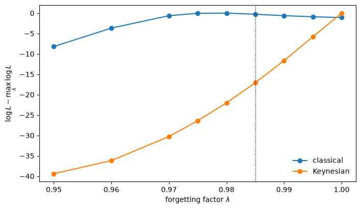
Compute the profile likelihood of the gain: for \(\lambda\) on a grid from \(.95\) to \(1\), rebuild the government’s beliefs and recommendations, re-estimate \((\theta, U^*, \rho_1, \rho_2)\), and plot the maximized \(\log L\) against \(\lambda\) for both identification schemes.
Note that \(\lambda = 1\) is least squares, with a gain that falls like \(1/t\).
Which values of \(\lambda\) do the data favor, and how does the answer bear on the book’s “mystery of why the stabilization was postponed”?
Solution
λ_grid = [0.95, 0.96, 0.97, 0.975, 0.98, 0.985, 0.99, 0.995, 1.0]
profile = {s: [] for s in 'CK'}
mean_K = []
for λ in λ_grid:
    for s in 'CK':
        g = government(data, s, λ=λ)
        profile[s].append(estimate(g)['loglik'])
        if s == 'K':
            mean_K.append(g['frame']['yhat'].loc['1973':'1979'].mean())

fig, ax = plt.subplots(figsize=(8, 4.5))
for s, label in [('C', 'classical'), ('K', 'Keynesian')]:
    ax.plot(λ_grid, np.array(profile[s]) - max(profile[s]), 'o-', label=label)
ax.axvline(0.985, color='k', ls=':', lw=1)
ax.set_xlabel(r'forgetting factor $\lambda$')
ax.set_ylabel(r'$\log L - \max_\lambda \log L$')
ax.legend(frameon=False)
plt.show()

print(" λ      log L (C)  log L (K)  K recommendation 1973-79")
for λ, lc, lk, m in zip(λ_grid, profile['C'], profile['K'], mean_K):
    print(f"{λ:5.3f}  {lc:9.1f}  {lk:9.1f}  {m:8.2f}")
 λ      log L (C)  log L (K)  K recommendation 1973-79
0.950     -595.5     -479.6      3.12
0.960     -591.0     -476.4      3.22
0.970     -588.0     -470.5      3.49
0.975     -587.4     -466.6      3.68
0.980     -587.3     -462.2      3.90
0.985     -587.6     -457.3      4.14
0.990     -588.0     -451.8      4.39
0.995     -588.2     -446.0      4.64
1.000     -588.4     -440.2      4.86
The classical likelihood is nearly flat for \(\lambda\) above .97, because the classical government recommends low inflation whatever its memory.
The Keynesian likelihood rises steadily as \(\lambda\) approaches one: the data prefer the government that discounts the past least.
The printed averages show why.
A government with a longer memory gives more weight to the 1950s and 1960s, when its regression showed a long-run tradeoff, so it activates the induction hypothesis later and recommends higher inflation in the 1970s, closer to the inflation that actually occurred.
Because the likelihood can reward a gain only by bringing the recommendations closer to actual inflation, it favors the slowest learner.
That is another way to state the book’s mystery: actual policy behaved as if it learned the natural-rate hypothesis later than the book’s constant-gain government did.
In the simulated economy of Exercise 91.7 the government really does follow its recommendations, and the likelihood recovers the true gain; here a preference for slow learning partly measures how far actual policy lagged behind the procedure.
Exercise 106.2
Sims [1988] gave his government a static Phillips curve, \(U_t = \gamma_0 y_t + \gamma_c + \varepsilon_t\), with no lags.
Estimate the static model (\(m_U = m_y = 0\)) under both identification schemes, and compare it with the distributed-lag model of the lecture.
For each of the four models, report the maximized \(\log L\), the average recommendation in 1973–1979, and the correlation between recommended and actual inflation.
Does the static classical model fail, and is it the lags or the direction of fit that matters more?
Solution
rows = []
for mU, my, lag_label in [(0, 0, 'static'), (1, 2, 'distributed lag')]:
    for s, label in [('C', 'classical'), ('K', 'Keynesian')]:
        g = government(data, s, mU=mU, my=my)
        f = g['frame'].loc['1958':]
        rows.append([lag_label, label, estimate(g)['loglik'],
                     f['yhat'].loc['1973':'1979'].mean(),
                     f[['y', 'yhat']].corr().iloc[0, 1]])
pd.DataFrame(rows, columns=['lags', 'scheme', 'log L', 'recommendation 1973-79',
                            'corr(recommended, actual)']
             ).set_index(['lags', 'scheme']).round(2)
| log L | recommendation 1973-79 | corr(recommended, actual) | ||
|---|---|---|---|---|
| lags | scheme | |||
| static | classical | -537.58 | 0.23 | -0.24 |
| Keynesian | -473.11 | 4.05 | 0.07 | |
| distributed lag | classical | -587.61 | -1.72 | 0.31 |
| Keynesian | -457.27 | 4.14 | 0.58 |
The static classical model does fail: it recommends inflation near zero in the 1970s, and its recommendations are negatively correlated with actual inflation.
But adding lags does not rescue the classical scheme: the distributed-lag classical government recommends even lower inflation, and its likelihood is lower than the static one’s.
The direction of fit matters more than the lags, and both Keynesian models fit far better than either classical model.
In a regression of unemployment on inflation, noise in quarterly inflation attenuates the coefficient on inflation, so a classical government sees only a weak tradeoff; inverting a regression of inflation on unemployment yields a steep one.
For the Keynesian scheme the lags matter too: the distributed-lag model has the higher likelihood, and its recommendations track actual inflation far more closely.
Only a distributed lag lets the government discover the induction hypothesis; a static Keynesian government has no lagged inflation in its model, so it cannot learn the natural-rate hypothesis in the Solow–Tobin form.
The book takes the two identification schemes, and their names, from King and Watson [1994], and it notes that the better fit of the Keynesian direction is what led the U.S. Phillips-curve literature to adopt it.
Exercise 106.3
Take the Keynesian government’s beliefs at the end of 1979Q2, just before Paul Volcker became chairman of the Federal Reserve.
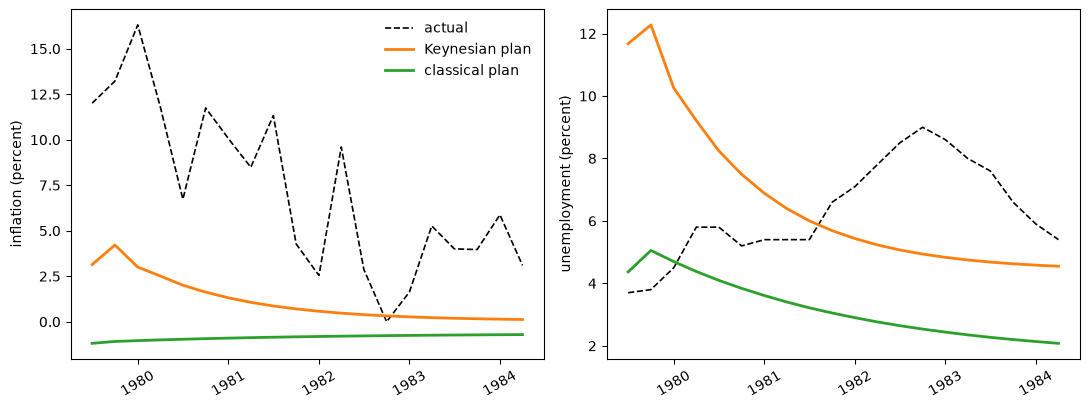
Compute the paths of inflation and unemployment that it planned for the next twenty quarters: the paths implied by its Phelps rule and its own estimated Phillips curve, with all future shocks set to zero, starting from the state in 1979Q3.
Do the same for the classical government, and plot both plans against what actually happened.
How does the Keynesian plan compare with the actual disinflation, and how large a rise in unemployment did each government expect to pay for it?
Solution
def planned_paths(g, date, H=20):
    "Inflation and unemployment the government planned from `date` on."
    t = g['frame'].index.get_loc(pd.Timestamp(date))
    β = g['coef'][t - 1]
    γ = β if g['scheme'] == 'C' else γ_of_β(β)
    h = phelps_h(γ, g['δ'], g['mU'], g['my'])
    A, B = lq_matrices(γ, g['mU'], g['my'])
    s = g['states'][t].copy()
    y_plan, U_plan = [], []
    for _ in range(H):
        y = h @ s
        y_plan.append(y)
        U_plan.append(γ[0] * y + γ[1:] @ s)
        s = A @ s + B[:, 0] * y
    index = g['frame'].index[t:t + H]
    return pd.DataFrame({'y': y_plan, 'U': U_plan}, index=index[:H])

date = '1979-07-01'
plans = {s: planned_paths(gov[s], date) for s in 'CK'}
actual = data.loc[date:].iloc[:20]

fig, axes = plt.subplots(1, 2, figsize=(11, 4.2))
for ax, var, ylabel in [(axes[0], 'y', 'inflation'), (axes[1], 'U', 'unemployment')]:
    ax.plot(actual.index, actual[var], 'k--', lw=1.2, label='actual')
    ax.plot(plans['K'].index, plans['K'][var], 'C1', lw=2, label='Keynesian plan')
    ax.plot(plans['C'].index, plans['C'][var], 'C2', lw=2, label='classical plan')
    ax.set_ylabel(f'{ylabel} (percent)')
    ax.tick_params(axis='x', rotation=30)
axes[0].legend(frameon=False)
plt.tight_layout()
plt.show()

print(f"1979Q2: inflation {data.loc['1979-04-01', 'y']:.1f}, "
      f"unemployment {data.loc['1979-04-01', 'U']:.1f}")
paths = {'Keynesian plan': plans['K'], 'classical plan': plans['C'], 'actual': actual}
print(f"{'':16s} {'y, 1st qtr':>10s} {'y, 4th qtr':>10s} {'y, 20th qtr':>11s} {'peak U':>7s}")
for label, p in paths.items():
    print(f"{label:16s} {p['y'].iloc[0]:10.1f} {p['y'].iloc[3]:10.1f} "
          f"{p['y'].iloc[-1]:11.1f} {p['U'].max():7.1f}")
1979Q2: inflation 12.9, unemployment 3.4
                 y, 1st qtr y, 4th qtr y, 20th qtr  peak U
Keynesian plan          3.1        2.5         0.1    12.3
classical plan         -1.2       -1.0        -0.7     5.1
actual                 12.0       11.8         3.1     9.0
On the eve of Volcker’s appointment the Keynesian government planned to cut inflation at once, from double digits to a few percent, and then to lower it slowly toward zero.
It expected the cut to be costly: unemployment in its plan jumps to well above its 1979 level and then declines slowly.
This is the pattern of the Phelps problem in chapter 5 of the book (Adaptive Expectations and the Phelps Problem), where the government “engineers a major recession and immediately brings inflation down more than half way toward its eventual limiting value.”
The classical government planned a mild deflation and expected it to cost little, because its estimated curve showed hardly any short-run effect of inflation on unemployment.
Actual policy moved more slowly than either plan: inflation stayed high for more than a year and reached its 1980s level only in 1982–1983, while the unemployment rate of white men rose to its peak at the end of 1982.
Both governments’ econometrics said disinflate now, and the Keynesian government recommended it even though it expected disinflation to be costly.
Neither would have accepted the argument, current in the late 1970s, that long lags in expectations made disinflation too costly to attempt.