64. Optimal Savings IV: Time Iteration#
In addition to what’s in Anaconda, this lecture will need the following libraries:
!pip install quantecon
64.1. Overview#
In this lecture, we introduce the core idea of time iteration: iterating on a guess of the optimal policy using the Euler equation.
This approach differs from the value function iteration we used in Optimal Savings III: Stochastic Returns, where we iterated on the value function itself.
Time iteration exploits the structure of the Euler equation to find the optimal policy directly, rather than computing the value function as an intermediate step.
The key advantage is computational efficiency: by working directly with the policy function, we can often solve problems faster than with value function iteration.
However, time iteration is not the most efficient Euler equation-based method available.
In Optimal Savings V: The Endogenous Grid Method, we’ll introduce the endogenous grid method (EGM), which provides an even more efficient way to solve the problem.
For now, our goal is to understand the basic mechanics of time iteration and how it leverages the Euler equation.
Let’s start with some imports:
import matplotlib.pyplot as plt
import numpy as np
from scipy.optimize import brentq
from typing import NamedTuple, Callable
64.2. The Euler Equation#
Our first step is to derive the Euler equation, which is a generalization of the Euler equation we obtained in Optimal Savings I: Cake Eating.
We take the model set out in Optimal Savings III: Stochastic Returns and add the following assumptions:
\(u\) and \(f\) are continuously differentiable and strictly concave
\(f(0) = 0\)
\(\lim_{c \to 0} u'(c) = \infty\) and \(\lim_{c \to \infty} u'(c) = 0\)
\(\lim_{k \to 0} f'(k) = \infty\) and \(\lim_{k \to \infty} f'(k) = 0\)
The last two conditions are usually called Inada conditions.
Recall the Bellman equation
Let \(v^*\) be the value function and let \(\sigma^*\) be the optimal consumption policy.
We know that \(\sigma^*\) is a \(v^*\)-greedy policy.
The conditions above imply that
\(\sigma^*\) is the unique optimal policy for the optimal savings problem
the optimal policy is continuous, strictly increasing and also interior, in the sense that \(0 < \sigma^*(x) < x\) for all strictly positive \(x\), and
the value function is strictly concave and continuously differentiable, with
The last result is called the envelope condition due to its relationship with the envelope theorem.
To see why (64.2) holds, write the Bellman equation in the equivalent form
Differentiating with respect to \(x\), and then evaluating at the optimum yields (64.2).
(Section 12.1 of EDTC contains full proofs of these results, and closely related discussions can be found in many other texts.)
Differentiability of the value function and interiority of the optimal policy imply that optimal consumption satisfies the first-order condition associated with (64.1), which is
Combining (64.2) and the first-order condition (64.3) gives the Euler equation
We can think of the Euler equation as a functional equation
over interior consumption policies \(\sigma\), one solution of which is the optimal policy \(\sigma^*\).
Our aim is to solve the functional equation (64.5) and hence obtain \(\sigma^*\).
64.2.1. The Coleman-Reffett Operator#
Recall the Bellman operator
Just as we introduced the Bellman operator to solve the Bellman equation, we will now introduce an operator over policies to help us solve the Euler equation.
This operator \(K\) will act on the set of all \(\sigma \in \Sigma\) that are continuous, strictly increasing and interior.
Henceforth we denote this set of policies by \(\mathscr P\)
The operator \(K\) takes as its argument a \(\sigma \in \mathscr P\) and
returns a new function \(K\sigma\), where \(K\sigma(x)\) is the \(c \in (0, x)\) that solves
We call this operator the Coleman-Reffett operator to acknowledge the work of [Coleman, 1990] and [Reffett, 1996].
In essence, \(K\sigma\) is the consumption policy that the Euler equation tells you to choose today when your future consumption policy is \(\sigma\).
The important thing to note about \(K\) is that, by construction, its fixed points coincide with solutions to the functional equation (64.5).
In particular, the optimal policy \(\sigma^*\) is a fixed point.
Indeed, for fixed \(x\), the value \(K\sigma^*(x)\) is the \(c\) that solves
In view of the Euler equation, this is exactly \(\sigma^*(x)\).
64.2.2. Is the Coleman-Reffett Operator Well Defined?#
In particular, is there always a unique \(c \in (0, x)\) that solves (64.7)?
The answer is yes, under our assumptions.
For any \(\sigma \in \mathscr P\), the right side of (64.7)
is continuous and strictly increasing in \(c\) on \((0, x)\)
diverges to \(+\infty\) as \(c \uparrow x\)
The left side of (64.7)
is continuous and strictly decreasing in \(c\) on \((0, x)\)
diverges to \(+\infty\) as \(c \downarrow 0\)
Sketching these curves and using the information above will convince you that they cross exactly once as \(c\) ranges over \((0, x)\).
With a bit more analysis, one can show in addition that \(K \sigma \in \mathscr P\) whenever \(\sigma \in \mathscr P\).
64.2.3. Comparison with VFI (Theory)#
It is possible to prove that there is a tight relationship between iterates of \(K\) and iterates of the Bellman operator.
Mathematically, \(T\) and \(K\) are topologically conjugate under a translation that involves differentiation in one direction and integration in the other.
This conjugacy implies that if iterates of one operator converge then so do iterates of the other, and vice versa.
Moreover, there is a sense in which they converge at the same rate, at least in theory.
However, it turns out that the operator \(K\) is more stable numerically and hence more efficient in the applications we consider.
This is because
\(K\) exploits additional structure because it uses first-order conditions, and
policies near the optimal policy have less curvature and hence are easier to approximate than value functions near the optimal value function.
Examples are given below.
64.3. Implementation#
Let’s turn to implementation.
Note
In this lecture we mainly focus on the algorithm, favoring clarity over efficiency in the code.
In later lectures we will optimize both the algorithm and the code.
As in Optimal Savings III: Stochastic Returns, we assume that
\(u(c) = \ln c\)
\(f(x-c) = (x-c)^{\alpha}\)
\(\phi\) is the distribution of \(\xi := \exp(\mu + \nu \zeta)\) when \(\zeta\) is standard normal
This allows us to compare our results to the analytical solutions we obtained in that lecture:
def v_star(x, α, β, μ):
    """
    True value function
    """
    c1 = np.log(1 - α * β) / (1 - β)
    c2 = (μ + α * np.log(α * β)) / (1 - α)
    c3 = 1 / (1 - β)
    c4 = 1 / (1 - α * β)
    return c1 + c2 * (c3 - c4) + c4 * np.log(x)

def σ_star(x, α, β):
    """
    True optimal policy
    """
    return (1 - α * β) * x
As discussed above, our plan is to solve the model using time iteration, which means iterating with the operator \(K\).
For this we need access to the functions \(u'\) and \(f, f'\).
We use the same Model structure from Optimal Savings III: Stochastic Returns.
class Model(NamedTuple):
    u: Callable        # utility function
    f: Callable        # production function
    β: float           # discount factor
    μ: float           # shock location parameter
    ν: float           # shock scale parameter
    grid: np.ndarray   # state grid
    shocks: np.ndarray # shock draws
    α: float = 0.4     # production function parameter
    u_prime: Callable = None        # derivative of utility
    f_prime: Callable = None        # derivative of production


def create_model(
        u: Callable,
        f: Callable,
        β: float = 0.96,
        μ: float = 0.0,
        ν: float = 0.1,
        grid_max: float = 4.0,
        grid_size: int = 120,
        shock_size: int = 250,
        seed: int = 1234,
        α: float = 0.4,
        u_prime: Callable = None,
        f_prime: Callable = None
    ) -> Model:
    """
    Creates an instance of the optimal savings model.
    """
    # Set up grid
    grid = np.linspace(1e-4, grid_max, grid_size)

    # Store shocks (with a seed, so results are reproducible)
    np.random.seed(seed)
    shocks = np.exp(μ + ν * np.random.randn(shock_size))

    return Model(u, f, β, μ, ν, grid, shocks, α, u_prime, f_prime)
Now we implement a method called euler_diff, which returns
def euler_diff(c: float, σ: np.ndarray, x: float, model: Model) -> float:
    """
    Set up a function such that the root with respect to c,
    given x and σ, is equal to Kσ(x).

    """

    # Unpack
    u, f, β, μ, ν, grid, shocks, α, u_prime, f_prime = model

    # Turn σ into a function via interpolation
    σ_func = lambda x: np.interp(x, grid, σ)

    # Now set up the function we need to find the root of.
    vals = u_prime(σ_func(f(x - c, α) * shocks)) * f_prime(x - c, α) * shocks
    return u_prime(c) - β * np.mean(vals)
The function euler_diff evaluates integrals by Monte Carlo and
approximates functions using linear interpolation.
We will use a root-finding algorithm to solve (64.8) for \(c\) given state \(x\) and \(σ\), the current guess of the policy.
Here’s the operator \(K\), that implements the root-finding step.
def K(σ: np.ndarray, model: Model) -> np.ndarray:
    """
    The Coleman-Reffett operator

    """

    # Unpack
    u, f, β, μ, ν, grid, shocks, α, u_prime, f_prime = model

    σ_new = np.empty_like(σ)
    for i, x in enumerate(grid):
        # Solve for optimal c at x
        c_star = brentq(euler_diff, 1e-10, x-1e-10, args=(σ, x, model))
        σ_new[i] = c_star

    return σ_new
64.3.1. Testing#
Let’s generate an instance and plot some iterates of \(K\), starting from \(σ(x) = x\).
# Define utility and production functions with derivatives
α = 0.4
u = lambda c: np.log(c)
u_prime = lambda c: 1 / c
f = lambda k, α: k**α
f_prime = lambda k, α: α * k**(α - 1)

model = create_model(u=u, f=f, α=α, u_prime=u_prime, f_prime=f_prime)
grid = model.grid

n = 15
σ = grid.copy()  # Set initial condition

fig, ax = plt.subplots()
lb = r'initial condition $\sigma(x) = x$'
ax.plot(grid, σ, color=plt.cm.jet(0), alpha=0.6, label=lb)

for i in range(n):
    σ = K(σ, model)
    ax.plot(grid, σ, color=plt.cm.jet(i / n), alpha=0.6)

# Update one more time and plot the last iterate in black
σ = K(σ, model)
ax.plot(grid, σ, color='k', alpha=0.8, label='last iterate')

ax.legend()

plt.show()
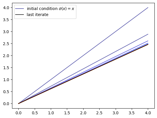
We see that the iteration process converges quickly to a limit that resembles the solution we obtained in Optimal Savings III: Stochastic Returns.
Here is a function called solve_model_time_iter that takes an instance of
Model and returns an approximation to the optimal policy,
using time iteration.
def solve_model_time_iter(
        model: Model,
        σ_init: np.ndarray,
        tol: float = 1e-5,
        max_iter: int = 1000,
        verbose: bool = True
    ) -> np.ndarray:
    """
    Solve the model using time iteration.

    """
    σ = σ_init
    error = tol + 1
    i = 0

    while error > tol and i < max_iter:
        σ_new = K(σ, model)
        error = np.max(np.abs(σ_new - σ))
        σ = σ_new
        i += 1
        if verbose:
            print(f"Iteration {i}, error = {error}")

    if i == max_iter:
        print("Warning: maximum iterations reached")

    return σ
Let’s call it:
# Unpack
grid = model.grid

σ_init = np.copy(grid)
σ = solve_model_time_iter(model, σ_init)
Iteration 1, error = 1.1098265895953756
Iteration 2, error = 0.27827989207957415
Iteration 3, error = 0.09312729948559406
Iteration 4, error = 0.034020038271351805
Iteration 5, error = 0.012820752818722525
Iteration 6, error = 0.004888081560539437
Iteration 7, error = 0.0018718902256105174
Iteration 8, error = 0.0007180512309568066
Iteration 9, error = 0.0002756205293255043
Iteration 10, error = 0.00010582190181418483
Iteration 11, error = 4.063319516811603e-05
Iteration 12, error = 1.560279084289462e-05
Iteration 13, error = 5.991419175455093e-06
Here is a plot of the resulting policy, compared with the true policy:
# Unpack
grid, α, β = model.grid, model.α, model.β

fig, ax = plt.subplots()

ax.plot(grid, σ, lw=2,
        alpha=0.8, label='approximate policy function')

ax.plot(grid, σ_star(grid, α, β), 'k--',
        lw=2, alpha=0.8, label='true policy function')

ax.legend()
plt.show()
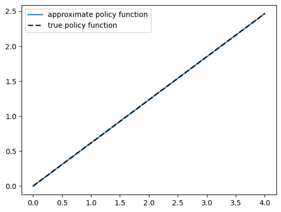
Again, the fit is excellent.
The maximal absolute deviation between the two policies is
# Unpack
grid, α, β = model.grid, model.α, model.β

np.max(np.abs(σ - σ_star(grid, α, β)))
np.float64(3.7348959489591493e-06)
Time iteration runs faster than value function iteration, as discussed in Optimal Savings III: Stochastic Returns.
This is because time iteration exploits differentiability and the first-order conditions, while value function iteration does not use this available structure.
At the same time, there is a variation of time iteration that runs even faster.
This is the endogenous grid method, which we will introduce in Optimal Savings V: The Endogenous Grid Method.
64.4. Exercises#
Exercise 64.1
Solve the optimal savings problem with CRRA utility
Set γ = 1.5.
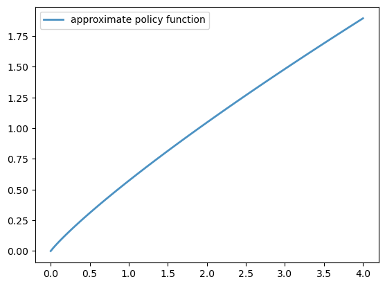
Compute and plot the optimal policy.
Solution
We define the CRRA utility function and its derivative.
γ = 1.5

def u_crra(c):
    return c**(1 - γ) / (1 - γ)

def u_prime_crra(c):
    return c**(-γ)

# Use the same production function as before
model_crra = create_model(u=u_crra, f=f, α=α,
                          u_prime=u_prime_crra, f_prime=f_prime)
Now we solve and plot the policy:
%%time
# Unpack
grid = model_crra.grid

σ_init = np.copy(grid)
σ = solve_model_time_iter(model_crra, σ_init)


fig, ax = plt.subplots()

ax.plot(grid, σ, lw=2,
        alpha=0.8, label='approximate policy function')

ax.legend()
plt.show()
Iteration 1, error = 1.449952719114732
Iteration 2, error = 0.3967698022828947
Iteration 3, error = 0.14845269076775747
Iteration 4, error = 0.06192954031818365
Iteration 5, error = 0.027017665601367424
Iteration 6, error = 0.012019070058330028
Iteration 7, error = 0.005393694573905705
Iteration 8, error = 0.0024299846499917788
Iteration 9, error = 0.0010967197524933692
Iteration 10, error = 0.0004953902833375601
Iteration 11, error = 0.0002238472234141753
Iteration 12, error = 0.0001011641350074921
Iteration 13, error = 4.572272482672446e-05
Iteration 14, error = 2.066580711579391e-05
Iteration 15, error = 9.340704450133686e-06
CPU times: user 634 ms, sys: 4.09 ms, total: 638 ms
Wall time: 637 ms