69. The Income Fluctuation Problem III: The Endogenous Grid Method#
GPU
This lecture was built using a machine with access to a GPU — although it will also run without one.
Google Colab has a free tier with GPUs that you can access as follows:
Click on the “play” icon top right
Select Colab
Set the runtime environment to include a GPU
69.1. Overview#
In this lecture we continue examining a version of the IFP from
The Income Fluctuation Problem I: Discretization and VFI and
The Income Fluctuation Problem II: Optimistic Policy Iteration.
We will make two changes.
Change the timing to one that is more efficient for our set up.
Use the endogenous grid method (EGM) to solve the model.
We use EGM because we know it to be fast and accurate from Optimal Savings VI: EGM with JAX.
The primary source for the technical details discussed below is [Ma et al., 2020].
Other references include [Deaton, 1991], [Den Haan, 2010], [Kuhn, 2013], [Rabault, 2002], [Reiter, 2009] and [Schechtman and Escudero, 1977].
In addition to what’s in Anaconda, this lecture will need the following libraries:
!pip install quantecon jax
We’ll also need the following imports:
import matplotlib.pyplot as plt
import numpy as np
import numba
from quantecon import MarkovChain
import jax
import jax.numpy as jnp
from typing import NamedTuple
69.2. The Household Problem#
Let’s write down the model and then discuss how to solve it.
69.2.1. Set-Up#
A household chooses a state-contingent consumption plan \(\{c_t\}_{t \geq 0}\) to maximize
subject to
Here
\(\beta \in (0,1)\) is the discount factor
\(a_t\) is asset holdings at time \(t\), with borrowing constraint \(a_t \geq 0\)
\(c_t\) is consumption
\(Y_t\) is non-capital income (wages, unemployment compensation, etc.)
\(R := 1 + r\), where \(r > 0\) is the interest rate on savings
The timing here is as follows:
At the start of period \(t\), the household observes current asset holdings \(a_t\).
The household chooses current consumption \(c_t\).
Savings \(s_t := a_t - c_t\) earns interest at rate \(r\).
Labor income \(Y_{t+1}\) is realized and time shifts to \(t+1\).
Non-capital income \(Y_t\) is given by \(Y_t = y(Z_t)\), where
\(\{Z_t\}\) is an exogenous state process, and
\(y\) is a function taking values in \(\mathbb{R}_+\).
We take \(\{Z_t\}\) to be a finite state Markov chain taking values in \(\mathsf Z\) with Markov matrix \(\Pi\).
Note
In previous lectures we used the more standard household budget constraint \(a_{t+1} + c_t \leq R a_t + Y_t\).
This setup, which is pervasive in quantitative economics, was developed for discretization.
It means that the control variable is also the next period state \(a_{t+1}\), which makes it straightforward to restrict assets to a finite grid.
But fixing the control to be the next period state forces us to include more information in the current state, which expands the size of the state space.
Moreover, aiming for discretization is not always a good idea, since it suffers heavily from the curse of dimensionality.
These ideas will become clearer in the next lecture.
We further assume that
\(\beta R < 1\)
\(u\) is smooth, strictly increasing and strictly concave with \(\lim_{c \to 0} u'(c) = \infty\) and \(\lim_{c \to \infty} u'(c) = 0\)
\(y(z) = \exp(z)\)
The asset space is \(\mathbb R_+\) and the state is the pair \((a,z) \in \mathsf S := \mathbb R_+ \times \mathsf Z\).
A feasible consumption path from \((a,z) \in \mathsf S\) is a consumption sequence \(\{c_t\}\) such that \(\{c_t\}\) and its induced asset path \(\{a_t\}\) satisfy
\((a_0, z_0) = (a, z)\)
the feasibility constraints in (69.1), and
adaptedness, which means that \(c_t\) is a function of random outcomes up to date \(t\) but not after.
The meaning of the third point is just that consumption at time \(t\) cannot be a function of outcomes are yet to be observed.
In fact, for this problem, consumption can be chosen optimally by taking it to be contingent only on the current state.
Optimality is defined below.
69.2.2. Value Function and Euler Equation#
The value function \(V \colon \mathsf S \to \mathbb{R}\) is defined by
where the maximization is overall feasible consumption paths from \((a,z)\).
An optimal consumption path from \((a,z)\) is a feasible consumption path from \((a,z)\) that maximizes (67.1).
To pin down such paths we can use a version of the Euler equation, which in the present setting is
with
When \(c_t\) hits the upper bound \(a_t\), the strict inequality \(u' (c_t) > \beta R \, \mathbb{E}_t u'(c_{t+1})\) can occur because \(c_t\) cannot increase sufficiently to attain equality.
The case \(c_t = 0\) never arises along the optimal path because \(u'(0) = \infty\).
69.2.3. Optimality Results#
As shown in [Ma et al., 2020],
For each \((a,z) \in \mathsf S\), a unique optimal consumption path from \((a,z)\) exists
This path is the unique feasible path from \((a,z)\) satisfying the Euler equations (69.3)-(69.4) and the transversality condition
Moreover, there exists an optimal consumption policy \(\sigma^* \colon \mathsf S \to \mathbb R_+\) such that the path from \((a,z)\) generated by
satisfies both the Euler equations (69.3)-(69.4) and (69.5), and hence is the unique optimal path from \((a,z)\).
Thus, to solve the optimization problem, we need to compute the policy \(\sigma^*\).
69.3. Computation#
We solve for the optimal consumption policy using time iteration and the endogenous grid method, which were previously discussed in
69.3.1. Solution Method#
We rewrite (69.4) to make it a statement about functions rather than random variables:
Here
\((u' \circ \sigma)(s) := u'(\sigma(s))\),
primes indicate next period states (as well as derivatives), and
\(\sigma\) is the unknown function.
The equality (69.6) holds at all interior choices, meaning \(\sigma(a, z) < a\).
We aim to find a fixed point \(\sigma\) of (69.6).
To do so we use the EGM.
Below we use the relationships \(a_t = c_t + s_t\) and \(a_{t+1} = R s_t + Y_{t+1}\).
We begin with an exogenous savings grid \(s_0 < s_1 < \cdots < s_m\) with \(s_0 = 0\).
We fix a current guess of the policy function \(\sigma\).
For each exogenous savings level \(s_i\) with \(i \geq 1\) and current state \(z_j\), we set
The Euler equation holds here because \(i \geq 1\) implies \(s_i > 0\) and hence consumption is interior.
For the boundary case \(s_0 = 0\) we set
We then obtain a corresponding endogenous grid of current assets via
Notice that, for each \(j\), we have \(a_{0j} = c_{0j} = 0\).
This anchors the interpolation at the correct value at the origin, since, without borrowing, consumption is zero when assets are zero.
Our next guess of the policy function, which we write as \(K\sigma\), is the linear interpolation of the interpolation points
for each \(j\).
(The number of one-dimensional linear interpolations is equal to the size of \(\mathsf Z\).)
69.4. NumPy Implementation#
In this section we’ll code up a NumPy version of the code that aims only for clarity, rather than efficiency.
Once we have it working, we’ll produce a JAX version that’s far more efficient and check that we obtain the same results.
We use the CRRA utility specification
69.4.1. Set Up#
Here we build a class called IFPNumPy that stores the model primitives.
The exogenous state process \(\{Z_t\}\) defaults to a two-state Markov chain with transition matrix \(\Pi\).
class IFPNumPy(NamedTuple):
    R: float                  # Gross interest rate R = 1 + r
    β: float                  # Discount factor
    γ: float                  # Preference parameter
    Π: np.ndarray             # Markov matrix for exogenous shock
    z_grid: np.ndarray        # Markov state values for Z_t
    s: np.ndarray             # Exogenous savings grid


def create_ifp(r=0.01,
               β=0.96,
               γ=1.5,
               Π=((0.6, 0.4),
                  (0.05, 0.95)),
               z_grid=(-10.0, np.log(2.0)),
               savings_grid_max=16,
               savings_grid_size=200):

    s = np.linspace(0, savings_grid_max, savings_grid_size)
    Π, z_grid = np.array(Π), np.array(z_grid)
    R = 1 + r
    assert R * β < 1, "Stability condition violated."
    return IFPNumPy(R, β, γ, Π, z_grid, s)
69.4.2. Solver#
Here is the operator \(K\) that transforms current guess \(\sigma\) into next period guess \(K\sigma\).
In practice, it takes in
a guess of optimal consumption values \(c_{ij}\), stored as
c_vecand a corresponding set of endogenous grid points \(a^e_{ij}\), stored as
a_vec
These are converted into a consumption policy \(a \mapsto \sigma(a, z_j)\) by linear interpolation of \((a^e_{ij}, c_{ij})\) over \(i\) for each \(j\).
Since there are no shocks to integrate out in this version of the model, we can compute (69.7) directly by summing over the finite state space \(\mathsf Z\).
@numba.jit
def K_numpy(
        c_in: np.ndarray,   # Initial guess of σ on grid endogenous grid
        a_in: np.ndarray,   # Initial endogenous grid
        ifp_numpy: IFPNumPy
    ) -> np.ndarray:
    """
    The Euler equation operator for the IFP model using the
    Endogenous Grid Method.

    This operator implements one iteration of the EGM algorithm to
    update the consumption policy function.

    """
    R, β, γ, Π, z_grid, s = ifp_numpy
    n_a, n_z = len(s), len(z_grid)
    c_out = np.zeros_like(c_in)
    u_prime = lambda c: c**(-γ)
    u_prime_inv = lambda c: c**(-1/γ)
    y = lambda z: np.exp(z)

    for i in range(1, n_a):  # Start from 1 for positive savings levels
        for j in range(n_z):

            # Compute Σ_z' u'(σ(R s_i + y(z'), z')) Π[z_j, z']
            expectation = 0.0
            for k in range(n_z):
                z_prime = z_grid[k]
                # Calculate next period assets
                next_a = R * s[i] + y(z_prime)
                # Interpolate to get σ(R s_i + y(z'), z')
                next_c = np.interp(next_a, a_in[:, k], c_in[:, k])
                # Weight by transition probability and add to the expectation
                expectation += u_prime(next_c) * Π[j, k]

            # Calculate updated c_{ij} values
            c_out[i, j] = u_prime_inv(β * R * expectation)

    a_out = c_out + s[:, None]
    return c_out, a_out
To solve the model we use a simple while loop.
def solve_model_numpy(
        ifp_numpy: IFPNumPy,
        c_init: np.ndarray,
        a_init: np.ndarray,
        tol: float = 1e-5,
        max_iter: int = 1_000
    ) -> np.ndarray:
    """
    Solve the model using time iteration with EGM.

    """
    c_in, a_in = c_init, a_init
    i = 0
    error = tol + 1

    while error > tol and i < max_iter:
        c_out, a_out = K_numpy(c_in, a_in, ifp_numpy)
        error = np.max(np.abs(c_out - c_in))
        i = i + 1
        c_in, a_in = c_out, a_out

    return c_out, a_out
Let’s road test the EGM code.
ifp_numpy = create_ifp()
R, β, γ, Π, z_grid, s = ifp_numpy
# Initial conditions -- agent consumes everything
a_init = s[:, None] * np.ones(len(z_grid))
c_init = a_init
# Solve from these initial conditions
c_vec, a_vec = solve_model_numpy(
    ifp_numpy, c_init, a_init
)
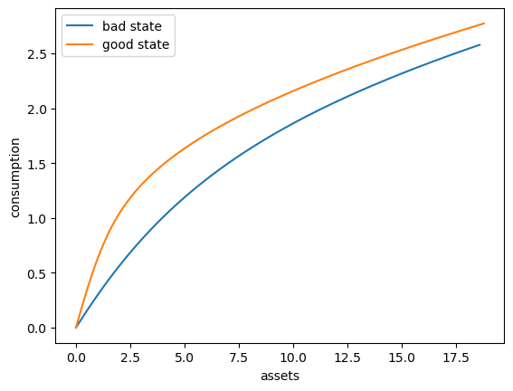
Here’s a plot of the optimal consumption policy for each \(z\) state
fig, ax = plt.subplots()

ax.plot(a_vec[:, 0], c_vec[:, 0], label='bad state')
ax.plot(a_vec[:, 1], c_vec[:, 1], label='good state')
ax.set(xlabel='assets', ylabel='consumption')
ax.legend()
plt.show()
69.5. JAX Implementation#
Now we write a more efficient JAX version, which can run on a GPU.
69.5.1. Set Up#
We start with a class called IFP that stores the model primitives.
class IFP(NamedTuple):
    R: float                  # Gross interest rate R = 1 + r
    β: float                  # Discount factor
    γ: float                  # Preference parameter
    Π: jnp.ndarray            # Markov matrix for exogenous shock
    z_grid: jnp.ndarray       # Markov state values for Z_t
    s: jnp.ndarray            # Exogenous savings grid


def create_ifp(r=0.01,
               β=0.94,
               γ=1.5,
               Π=((0.6, 0.4),
                  (0.05, 0.95)),
               z_grid=(-10.0, jnp.log(2.0)),
               savings_grid_max=16,
               savings_grid_size=200):

    s = jnp.linspace(0, savings_grid_max, savings_grid_size)
    Π, z_grid = jnp.array(Π), jnp.array(z_grid)
    R = 1 + r
    assert R * β < 1, "Stability condition violated."
    return IFP(R, β, γ, Π, z_grid, s)
69.5.2. Solver#
Here is the operator \(K\) that transforms current guess \(\sigma\) into next period guess \(K\sigma\).
def K(
        c_in: jnp.ndarray,
        a_in: jnp.ndarray,
        ifp: IFP
    ) -> jnp.ndarray:
    """
    The Euler equation operator for the IFP model using the
    Endogenous Grid Method.

    This operator implements one iteration of the EGM algorithm to
    update the consumption policy function.

    """
    R, β, γ, Π, z_grid, s = ifp
    n_z = len(z_grid)
    z_indices = jnp.arange(n_z)
    u_prime = lambda c: c**(-γ)
    u_prime_inv = lambda c: c**(-1/γ)
    y = lambda z: jnp.exp(z)

    def compute_c(i, j):
        " Computes consumption for one (i, j) pair where i >= 1. "

        def compute_mu_k(k):
            " Given i, compute marginal utility u'(σ(R s_i + y(z_k), z_k)) "
            next_a = R * s[i] + y(z_grid[k])
            # Interpolate to get σ(R * s_i + y(z_k), z_k)
            next_c = jnp.interp(next_a, a_in[:, k], c_in[:, k])
            # Return u'(σ(R * s_i + y(z_k), z_k))
            return u_prime(next_c)

        # Compute marginal utility u'(σ(R * s_i + y(z_k), z_k)) for all k
        mu_values = jax.vmap(compute_mu_k)(z_indices)
        # Compute expectation Σ_k u'(σ(...)) * Π[j, k]
        expectation = jnp.sum(mu_values * Π[j, :])
        # Invert to get consumption c_{ij} at (s_i, z_j)
        return u_prime_inv(β * R * expectation)

    # vmap over j for each i
    compute_c_i = jax.vmap(compute_c, in_axes=(None, 0))
    # vmap over i
    compute_c = jax.vmap(lambda i: compute_c_i(i, z_indices))
    # Compute consumption for i >= 1
    c_out_interior = compute_c(jnp.arange(1, len(s)))
    # For i = 0, set consumption to 0
    c_out_boundary = jnp.zeros((1, n_z))
    # Concatenate boundary and interior
    c_out = jnp.concatenate([c_out_boundary, c_out_interior], axis=0)
    # Compute endogenous asset grid a_{ij} = c_{ij} + s_i
    a_out = c_out + s[:, None]
    return c_out, a_out
Here’s a jit-accelerated iterative routine to solve the model using this operator.
@jax.jit
def solve_model(
        ifp: IFP,
        c_init: jnp.ndarray,  # Initial guess of σ on grid endogenous grid
        a_init: jnp.ndarray,  # Initial endogenous grid
        tol: float = 1e-5,
        max_iter: int = 1000
    ) -> jnp.ndarray:
    """
    Solve the model using time iteration with EGM.

    """

    def condition(loop_state):
        c_in, a_in, i, error = loop_state
        return (error > tol) & (i < max_iter)

    def body(loop_state):
        c_in, a_in, i, error = loop_state
        c_out, a_out = K(c_in, a_in, ifp)
        error = jnp.max(jnp.abs(c_out - c_in))
        i += 1
        return c_out, a_out, i, error

    i, error = 0, tol + 1
    initial_state = (c_init, a_init, i, error)
    final_loop_state = jax.lax.while_loop(condition, body, initial_state)
    c_out, a_out, i, error = final_loop_state

    return c_out, a_out
69.5.3. Test run#
Let’s road test the EGM code.
ifp = create_ifp()
R, β, γ, Π, z_grid, s = ifp
# Set initial conditions where the agent consumes everything
a_init = s[:, None] * jnp.ones(len(z_grid))
c_init = a_init
# Solve starting from these initial conditions
c_vec_jax, a_vec_jax = solve_model(ifp, c_init, a_init)
To verify the correctness of our JAX implementation, let’s compare it with the NumPy version we developed earlier.
# Compare the results
max_c_diff = np.max(np.abs(np.array(c_vec) - c_vec_jax))
max_ae_diff = np.max(np.abs(np.array(a_vec) - a_vec_jax))

print(f"Maximum difference in consumption policy: {max_c_diff:.2e}")
print(f"Maximum difference in asset grid:        {max_ae_diff:.2e}")
Maximum difference in consumption policy: 4.45e-01
Maximum difference in asset grid:        4.45e-01
These numbers confirm that we are computing essentially the same policy using the two approaches.
69.5.4. Timing#
Now let’s compare the execution time between NumPy and JAX implementations.
import time

# Set up initial conditions for NumPy version
s_np = np.array(s)
z_grid_np = np.array(z_grid)
a_init_np = s_np[:, None] * np.ones(len(z_grid_np))
c_init_np = a_init_np.copy()

# Set up initial conditions for JAX version
a_init_jx = s[:, None] * jnp.ones(len(z_grid))
c_init_jx = a_init_jx

# Time NumPy version
start = time.time()
c_vec_np, a_vec_np = solve_model_numpy(ifp_numpy, c_init_np, a_init_np)
numpy_time = time.time() - start

# Time JAX version (with compilation)
start = time.time()
c_vec_jx, a_vec_jx = solve_model(ifp, c_init_jx, a_init_jx)
c_vec_jx.block_until_ready()
jax_time_with_compile = time.time() - start

# Time JAX version (without compilation - second run)
start = time.time()
c_vec_jx, a_vec_jx = solve_model(ifp, c_init_jx, a_init_jx)
c_vec_jx.block_until_ready()
jax_time = time.time() - start

print(f"NumPy time:                 {numpy_time:.4f} seconds")
print(f"JAX time (with compile):    {jax_time_with_compile:.4f} seconds")
print(f"JAX time (without compile): {jax_time:.4f} seconds")
print(f"Speedup (NumPy/JAX):        {numpy_time/jax_time:.2f}x")
NumPy time:                 0.0209 seconds
JAX time (with compile):    0.0100 seconds
JAX time (without compile): 0.0097 seconds
Speedup (NumPy/JAX):        2.16x
The JAX implementation is faster due to JIT compilation and GPU/TPU acceleration (if available).
Here’s a plot of the optimal policy for each \(z\) state
fig, ax = plt.subplots()
ax.plot(a_vec[:, 0], c_vec[:, 0], label='bad state')
ax.plot(a_vec[:, 1], c_vec[:, 1], label='good state')
ax.set(xlabel='assets', ylabel='consumption')
ax.legend()
plt.show()
69.5.5. Dynamics#
To begin to understand the long run asset levels held by households under the default parameters, let’s look at the 45 degree diagram showing the law of motion for assets under the optimal consumption policy.
fig, ax = plt.subplots()

y = lambda z: jnp.exp(z)

def y_bar(k):
    """
    Taking z = z_grid[k], compute

            E_z Y' = Σ_{z'} y(z') Π[z, z']

    This is the expectation of Y_{t+1} given Z_t = z.
    """
    # Compute y(z') for all z'
    y_values = jax.vmap(y)(z_grid)
    # Weight by transition probabilities and sum
    return jnp.sum(y_values * Π[k, :])

for k, label in zip((0, 1), ('low income', 'high income')):
    # Interpolate consumption policy on the savings grid
    c_on_grid = jnp.interp(s, a_vec[:, k], c_vec[:, k])
    ax.plot(s, R * (s - c_on_grid) + y_bar(k) , label=label)

ax.plot(s, s, 'k--')
ax.set(xlabel='current assets', ylabel='next period assets')

ax.legend()
plt.show()
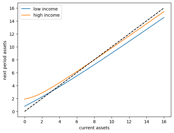
The unbroken lines show the update function for assets at each \(z\), which is
where
is the expected labor income conditional on current state \(z\).
The dashed line is the 45 degree line.
The figure suggests that, on average, the dynamics will be stable — assets do not diverge even in the highest state.
This turns out to be true: there is a unique stationary distribution of assets.
For details see [Ma et al., 2020]
This stationary distribution represents the long run dispersion of assets across households when households have idiosyncratic shocks.
69.5.6. A Sanity Check#
One way to check our results is to
set labor income to zero in each state and
set the gross interest rate \(R\) to unity.
In this case, our income fluctuation problem is just a CRRA cake eating problem.
Then the value function and optimal consumption policy are given by
def c_star(x, β, γ):
    return (1 - β ** (1/γ)) * x


def v_star(x, β, γ):
    return (1 - β**(1 / γ))**(-γ) * (x**(1-γ) / (1-γ))
Let’s see if we match up:
ifp_cake_eating = create_ifp(r=0.0, z_grid=(-jnp.inf, -jnp.inf))
R, β, γ, Π, z_grid, s = ifp_cake_eating
a_init = s[:, None] * jnp.ones(len(z_grid))
c_init = a_init
c_vec, a_vec = solve_model(ifp_cake_eating, c_init, a_init)

fig, ax = plt.subplots()
ax.plot(a_vec[:, 0], c_vec[:, 0], label='numerical')
ax.plot(a_vec[:, 0],
        c_star(a_vec[:, 0], ifp_cake_eating.β, ifp_cake_eating.γ),
        '--', label='analytical')
ax.set(xlabel='assets', ylabel='consumption')
ax.legend()
plt.show()
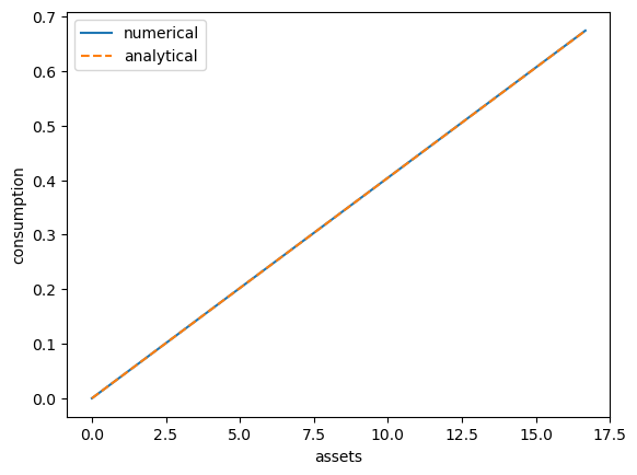
This looks pretty good.
69.6. Simulation#
Let’s return to the default model and study the stationary distribution of assets.
Our plan is to run a large number of households forward for \(T\) periods and then histogram the cross-sectional distribution of assets.
Set num_households=50_000, T=500.
First we write a function to run a single household forward in time and record the final value of assets.
The function takes a solution pair c_vec and a_vec, understanding them
as representing an optimal policy associated with a given model ifp
@jax.jit
def simulate_household(
        key, a_0, z_idx_0, c_vec, a_vec, ifp, T
    ):
    """
    Simulates a single household for T periods to approximate the stationary
    distribution of assets.

    - key is the state of the random number generator
    - ifp is an instance of IFP
    - c_vec, a_vec are the optimal consumption policy, endogenous grid for ifp

    """
    R, β, γ, Π, z_grid, s = ifp
    n_z = len(z_grid)

    y = lambda z: jnp.exp(z)
    σ = lambda a, z_idx: jnp.interp(a, a_vec[:, z_idx], c_vec[:, z_idx])

    # Simulate forward T periods
    def update(t, state):
        a, z_idx = state
        # Draw next shock z' from Π[z, z']
        current_key = jax.random.fold_in(key, t)
        z_next_idx = jax.random.choice(current_key, n_z, p=Π[z_idx]).astype(jnp.int32)
        z_next = z_grid[z_next_idx]
        # Update assets: a' = R * (a - c) + Y'
        a_next = R * (a - σ(a, z_idx)) + y(z_next)
        # Return updated state
        return a_next, z_next_idx

    initial_state = a_0, z_idx_0
    final_state = jax.lax.fori_loop(0, T, update, initial_state)
    a_final, _ = final_state
    return a_final
Now we write a function to simulate many households in parallel.
def compute_asset_stationary(
        c_vec, a_vec, ifp, num_households=50_000, T=500, seed=1234
    ):
    """
    Simulates num_households households for T periods to approximate
    the stationary distribution of assets.

    Returns the final cross-section of asset holdings.

    - ifp is an instance of IFP
    - c_vec, a_vec are the optimal consumption policy and endogenous grid.

    """
    R, β, γ, Π, z_grid, s = ifp
    n_z = len(z_grid)

    # Create interpolation function for consumption policy
    # Interpolate on the endogenous grid
    σ = lambda a, z_idx: jnp.interp(a, a_vec[:, z_idx], c_vec[:, z_idx])

    # Start with assets = savings_grid_max / 2
    a_0_vector = jnp.full(num_households, s[-1] / 2)
    # Initialize the exogenous state of each household
    z_idx_0_vector = jnp.zeros(num_households).astype(jnp.int32)

    # Vectorize over many households
    key = jax.random.PRNGKey(seed)
    keys = jax.random.split(key, num_households)
    # Vectorize simulate_household in (key, a_0, z_idx_0)
    sim_all_households = jax.vmap(
        simulate_household, in_axes=(0, 0, 0, None, None, None, None)
    )
    assets = sim_all_households(keys, a_0_vector, z_idx_0_vector, c_vec, a_vec, ifp, T)

    return np.array(assets)
Now we call the function, generate the asset distribution and histogram it:
ifp = create_ifp()
R, β, γ, Π, z_grid, s = ifp
a_init = s[:, None] * jnp.ones(len(z_grid))
c_init = a_init
c_vec, a_vec = solve_model(ifp, c_init, a_init)
assets = compute_asset_stationary(c_vec, a_vec, ifp)

fig, ax = plt.subplots()
ax.hist(assets, bins=20, alpha=0.5, density=True)
ax.set(xlabel='assets', title="Cross-sectional distribution of wealth")
plt.show()
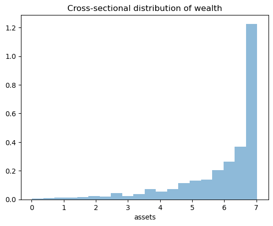
The wealth distribution looks very different to a typical wealth distribution in the data.
For one thing it is left-skewed rather than right-skewed.
In fact there is essentially no right-hand tail, even though real-world wealth distributions have long right-hand tails.
We’ll do our best to fix these issues in the next few lectures.