37. Von Neumann Growth Model (and a Generalization)#
This lecture uses the class Neumann to calculate key objects of a
linear growth model of John von Neumann [von Neumann, 1937] that was generalized by
Kemeny, Morgenstern and Thompson [Kemeny et al., 1956].
Objects of interest are the maximal expansion rate (\(\alpha\)), the interest factor (\(β\)), the optimal intensities (\(x\)), and prices (\(p\)).
In addition to watching how the towering mind of John von Neumann formulated an equilibrium model of price and quantity vectors in balanced growth, this lecture shows how fruitfully to employ the following important tools:
a zero-sum two-player game
linear programming
the Perron-Frobenius theorem
We’ll begin with some imports:
import numpy as np
import matplotlib.pyplot as plt
from scipy.optimize import fsolve, linprog
from textwrap import dedent

np.set_printoptions(precision=2)
The code below provides the Neumann class
class Neumann:

    """
    This class describes the Generalized von Neumann growth model as it was
    discussed in Kemeny et al. (1956, ECTA) and Gale (1960, Chapter 9.5):

    Let:
    n ... number of goods
    m ... number of activities
    A ... input matrix is m-by-n
        a_{i,j} - amount of good j consumed by activity i
    B ... output matrix is m-by-n
        b_{i,j} - amount of good j produced by activity i

    x ... intensity vector (m-vector) with non-negative entries
        x'B - the vector of goods produced
        x'A - the vector of goods consumed
    p ... price vector (n-vector) with non-negative entries
        Bp - the revenue vector for every activity
        Ap - the cost of each activity

    Both A and B have non-negative entries. Moreover, we assume that
    (1) Assumption I (every good which is consumed is also produced):
        for all j, b_{.,j} > 0, i.e. at least one entry is strictly positive
    (2) Assumption II (no free lunch):
        for all i, a_{i,.} > 0, i.e. at least one entry is strictly positive

    Parameters
    ----------
    A : array_like or scalar(float)
        Part of the state transition equation.  It should be `n x n`
    B : array_like or scalar(float)
        Part of the state transition equation.  It should be `n x k`
    """

    def __init__(self, A, B):

        self.A, self.B = list(map(self.convert, (A, B)))
        self.m, self.n = self.A.shape

        # Check if (A, B) satisfy the basic assumptions
        assert self.A.shape == self.B.shape, 'The input and output matrices \
              must have the same dimensions!'
        assert (self.A >= 0).all() and (self.B >= 0).all(), 'The input and \
              output matrices must have only non-negative entries!'

        # (1) Check whether Assumption I is satisfied:
        if (np.sum(B, 0) <= 0).any():
            self.AI = False
        else:
            self.AI = True

        # (2) Check whether Assumption II is satisfied:
        if (np.sum(A, 1) <= 0).any():
            self.AII = False
        else:
            self.AII = True

    def __repr__(self):
        return self.__str__()

    def __str__(self):

        me = """
        Generalized von Neumann expanding model:
          - number of goods          : {n}
          - number of activities     : {m}

        Assumptions:
          - AI:  every column of B has a positive entry    : {AI}
          - AII: every row of A has a positive entry       : {AII}

        """
        # Irreducible                                       : {irr}
        return dedent(me.format(n=self.n, m=self.m,
                                AI=self.AI, AII=self.AII))

    def convert(self, x):
        """
        Convert array_like objects (lists of lists, floats, etc.) into
        well-formed 2D NumPy arrays
        """
        return np.atleast_2d(np.asarray(x))


    def bounds(self):
        """
        Calculate the trivial upper and lower bounds for alpha (expansion rate)
        and beta (interest factor). See the proof of Theorem 9.8 in Gale (1960)
        """

        n, m = self.n, self.m
        A, B = self.A, self.B

        f = lambda α: ((B - α * A) @ np.ones((n, 1))).max()
        g = lambda β: (np.ones((1, m)) @ (B - β * A)).min()

        UB = fsolve(f, 1).item()  # Upper bound for α, β
        LB = fsolve(g, 2).item()  # Lower bound for α, β

        return LB, UB


    def zerosum(self, γ, dual=False):
        """
        Given gamma, calculate the value and optimal strategies of a
        two-player zero-sum game given by the matrix

                M(gamma) = B - gamma * A

        Row player maximizing, column player minimizing

        Zero-sum game as an LP (primal --> α)

            max (0', 1) @ (x', v)
            subject to
            [-M', ones(n, 1)] @ (x', v)' <= 0
            (x', v) @ (ones(m, 1), 0) = 1
            (x', v) >= (0', -inf)

        Zero-sum game as an LP (dual --> beta)

            min (0', 1) @ (p', u)
            subject to
            [M, -ones(m, 1)] @ (p', u)' <= 0
            (p', u) @ (ones(n, 1), 0) = 1
            (p', u) >= (0', -inf)

        Outputs:
        --------
        value: scalar
            value of the zero-sum game

        strategy: vector
            if dual = False, it is the intensity vector,
            if dual = True, it is the price vector
        """

        A, B, n, m = self.A, self.B, self.n, self.m
        M = B - γ * A

        if dual == False:
            # Solve the primal LP (for details see the description)
            # (1) Define the problem for v as a maximization (linprog minimizes)
            c = np.hstack([np.zeros(m), -1])

            # (2) Add constraints :
            # ... non-negativity constraints
            bounds = tuple(m * [(0, None)] + [(None, None)])
            # ... inequality constraints
            A_iq = np.hstack([-M.T, np.ones((n, 1))])
            b_iq = np.zeros((n, 1))
            # ... normalization
            A_eq = np.hstack([np.ones(m), 0]).reshape(1, m + 1)
            b_eq = 1

            res = linprog(c, A_ub=A_iq, b_ub=b_iq, A_eq=A_eq, b_eq=b_eq,
                          bounds=bounds)

        else:
            # Solve the dual LP (for details see the description)
            # (1) Define the problem for v as a maximization (linprog minimizes)
            c = np.hstack([np.zeros(n), 1])

            # (2) Add constraints :
            # ... non-negativity constraints
            bounds = tuple(n * [(0, None)] + [(None, None)])
            # ... inequality constraints
            A_iq = np.hstack([M, -np.ones((m, 1))])
            b_iq = np.zeros((m, 1))
            # ... normalization
            A_eq = np.hstack([np.ones(n), 0]).reshape(1, n + 1)
            b_eq = 1

            res = linprog(c, A_ub=A_iq, b_ub=b_iq, A_eq=A_eq, b_eq=b_eq,
                          bounds=bounds)

        if res.status != 0:
            print(res.message)

        # Pull out the required quantities
        value = res.x[-1]
        strategy = res.x[:-1]

        return value, strategy


    def expansion(self, tol=1e-8, maxit=1000):
        """
        The algorithm used here is described in Hamburger-Thompson-Weil
        (1967, ECTA). It is based on a simple bisection argument and utilizes
        the idea that for a given γ (= α or β), the matrix "M = B - γ * A"
        defines a two-player zero-sum game, where the optimal strategies are
        the (normalized) intensity and price vector.

        Outputs:
        --------
        alpha: scalar
            optimal expansion rate
        """

        LB, UB = self.bounds()

        for iter in range(maxit):

            γ = (LB + UB) / 2
            ZS = self.zerosum(γ=γ)
            V = ZS[0]     # value of the game with γ

            if V >= 0:
                LB = γ
            else:
                UB = γ

            if abs(UB - LB) < tol:
                γ = (UB + LB) / 2
                x = self.zerosum(γ=γ)[1]
                p = self.zerosum(γ=γ, dual=True)[1]
                break

        return γ, x, p

    def interest(self, tol=1e-8, maxit=1000):
        """
        The algorithm used here is described in Hamburger-Thompson-Weil
        (1967, ECTA). It is based on a simple bisection argument and utilizes
        the idea that for a given gamma (= alpha or beta),
        the matrix "M = B - γ * A" defines a two-player zero-sum game,
        where the optimal strategies are the (normalized) intensity and price
        vector

        Outputs:
        --------
        beta: scalar
            optimal interest rate
        """

        LB, UB = self.bounds()

        for iter in range(maxit):
            γ = (LB + UB) / 2
            ZS = self.zerosum(γ=γ, dual=True)
            V = ZS[0]

            if V > 0:
                LB = γ
            else:
                UB = γ

            if abs(UB - LB) < tol:
                γ = (UB + LB) / 2
                p = self.zerosum(γ=γ, dual=True)[1]
                x = self.zerosum(γ=γ)[1]
                break

        return γ, x, p
37.1. Notation#
We use the following notation.
\(\mathbf{0}\) denotes a vector of zeros.
We call an \(n\)-vector positive and write \(x\gg \mathbf{0}\) if \(x_i>0\) for all \(i=1,2,\dots,n\).
We call a vector non-negative and write \(x\geq \mathbf{0}\) if \(x_i\geq 0\) for all \(i=1,2,\dots,n\).
We call a vector semi-positive written \(x > \mathbf{0}\) if \(x\geq \mathbf{0}\) and \(x\neq \mathbf{0}\).
For two conformable vectors \(x\) and \(y\), \(x\gg y\), \(x\geq y\) and \(x> y\) mean \(x-y\gg \mathbf{0}\), \(x-y \geq \mathbf{0}\), and \(x-y > \mathbf{0}\), respectively.
We let all vectors in this lecture be column vectors; \(x^\top\) denotes the transpose of \(x\) (i.e., a row vector).
Let \(\iota_n\) denote a column vector composed of \(n\) ones, i.e. \(\iota_n = (1,1,\dots,1)^\top\).
Let \(e^i\) denote a vector (of arbitrary size) containing zeros except for the \(i\) th position where it is one.
We denote matrices by capital letters. For an arbitrary matrix \(A\), \(a_{i,j}\) represents the entry in its \(i\) th row and \(j\) th column.
\(a_{\cdot j}\) and \(a_{i\cdot}\) denote the \(j\) th column and \(i\) th row of \(A\), respectively.
37.2. Model Ingredients and Assumptions#
A pair \((A,B)\) of \(m\times n\) non-negative matrices defines an economy.
\(m\) is the number of activities (or sectors)
\(n\) is the number of goods (produced and/or consumed)
\(A\) is called the input matrix; \(a_{i,j}\) denotes the amount of good \(j\) consumed by activity \(i\)
\(B\) is called the output matrix; \(b_{i,j}\) represents the amount of good \(j\) produced by activity \(i\)
Two key assumptions restrict economy \((A,B)\):
Assumption 37.1 (every good that is consumed is also produced)
Assumption 37.2 (no free lunch)
A semi-positive intensity \(m\)-vector \(x\) denotes levels at which activities are operated.
Therefore,
vector \(x^\top A\) gives the total amount of goods used in production
vector \(x^\top B\) gives total outputs
An economy \((A,B)\) is said to be productive, if there exists a non-negative intensity vector \(x \geq 0\) such that \(x^\top B > x^\top A\).
The semi-positive \(n\)-vector \(p\) contains prices assigned to the \(n\) goods.
The \(p\) vector implies cost and revenue vectors
the vector \(Ap\) tells costs of the vector of activities
the vector \(Bp\) tells revenues from the vector of activities
Satisfaction of a property of an input-output pair \((A,B)\) called irreducibility (or indecomposability) determines whether an economy can be decomposed into multiple “sub-economies”.
Definition 37.1
For an economy \((A,B)\), the set of goods \(S\subset \{1,2,\dots,n\}\) is called an independent subset if it is possible to produce every good in \(S\) without consuming goods from outside \(S\).
Formally, the set \(S\) is independent if \(\exists T\subset \{1,2,\dots,m\}\) (a subset of activities) such that \(a_{i,j}=0\), \(\forall i\in T\) and \(j\in S^c\) and for all \(j\in S\), \(\exists i\in T\) for which \(b_{i,j}>0\).
The economy is irreducible if there are no proper independent subsets.
We study two examples, both in Chapter 9.6 of Gale [Gale, 1989]
# (1) Irreducible (A, B) example: α_0 = β_0
A1 = np.array([[0, 1, 0, 0],
               [1, 0, 0, 1],
               [0, 0, 1, 0]])

B1 = np.array([[1, 0, 0, 0],
               [0, 0, 2, 0],
               [0, 1, 0, 1]])

# (2) Reducible (A, B) example: β_0 < α_0
A2 = np.array([[0, 1, 0, 0, 0, 0],
               [1, 0, 1, 0, 0, 0],
               [0, 0, 0, 1, 0, 0],
               [0, 0, 1, 0, 0, 1],
               [0, 0, 0, 0, 1, 0]])

B2 = np.array([[1, 0, 0, 1, 0, 0],
               [0, 1, 0, 0, 0, 0],
               [0, 0, 1, 0, 0, 0],
               [0, 0, 0, 0, 2, 0],
               [0, 0, 0, 1, 0, 1]])
The following code sets up our first Neumann economy or Neumann
instance
n1 = Neumann(A1, B1)
n1
Generalized von Neumann expanding model:
  - number of goods          : 4
  - number of activities     : 3

Assumptions:
  - AI:  every column of B has a positive entry    : True
  - AII: every row of A has a positive entry       : True
Here is a second instance of a Neumann economy
n2 = Neumann(A2, B2)
n2
Generalized von Neumann expanding model:
  - number of goods          : 6
  - number of activities     : 5

Assumptions:
  - AI:  every column of B has a positive entry    : True
  - AII: every row of A has a positive entry       : True
37.3. Dynamic Interpretation#
Attach a time index \(t\) to the preceding objects, regard an economy as a dynamic system, and study sequences
An interesting special case holds the technology process constant and investigates the dynamics of quantities and prices only.
Accordingly, in the rest of this lecture, we assume that \((A_t,B_t)=(A,B)\) for all \(t\geq 0\).
A crucial element of the dynamic interpretation involves the timing of production.
We assume that production (consumption of inputs) takes place in period \(t\), while the consequent output materializes in period \(t+1\), i.e., consumption of \(x_{t}^\top A\) in period \(t\) results in \(x^\top_{t}B\) amounts of output in period \(t+1\).
These timing conventions imply the following feasibility condition:
which asserts that no more goods can be used today than were produced yesterday.
Accordingly, \(Ap_t\) tells the costs of production in period \(t\) and \(Bp_t\) tells revenues in period \(t+1\).
37.3.1. Balanced Growth#
We follow John von Neumann in studying “balanced growth”.
Let \(./\) denote an elementwise division of one vector by another and let \(\alpha >0\) be a scalar.
Then balanced growth is a situation in which
With balanced growth, the law of motion of \(x\) is evidently \(x_{t+1}=\alpha x_t\) and so we can rewrite the feasibility constraint as
In the same spirit, define \(\beta\in\mathbb{R}\) as the interest factor per unit of time.
We assume that it is always possible to earn a gross return equal to the constant interest factor \(\beta\) by investing “outside the model”.
Under this assumption about outside investment opportunities, a no-arbitrage condition gives rise to the following (no profit) restriction on the price sequence:
This says that production cannot yield a return greater than that offered by the outside investment opportunity (here we compare values in period \(t+1\)).
The balanced growth assumption allows us to drop time subscripts and conduct an analysis purely in terms of a time-invariant growth rate \(\alpha\) and interest factor \(\beta\).
37.4. Duality#
Two problems are connected by a remarkable dual relationship between technological and valuation characteristics of the economy:
Definition 37.2
The technological expansion problem (TEP) for the economy \((A,B)\) is to find a semi-positive \(m\)-vector \(x>0\) and a number \(\alpha\in\mathbb{R}\) that satisfy
Theorem 9.3 of David Gale’s book [Gale, 1989] asserts that if Assumption 37.1 and Assumption 37.2 are both satisfied, then a maximum value of \(\alpha\) exists and that it is positive.
The maximal value is called the technological expansion rate and is denoted by \(\alpha_0\). The associated intensity vector \(x_0\) is the optimal intensity vector.
Definition 37.3
The economic expansion problem (EEP) for \((A,B)\) is to find a semi-positive \(n\)-vector \(p>0\) and a number \(\beta\in\mathbb{R}\) that satisfy
Assumption 37.1 and Assumption 37.2 imply existence of a minimum value \(\beta_0>0\) called the economic expansion rate.
The corresponding price vector \(p_0\) is the optimal price vector.
Because the criterion functions in the technological expansion problem and the economical expansion problem are both linearly homogeneous, the optimality of \(x_0\) and \(p_0\) are defined only up to a positive scale factor.
For convenience (and to emphasize a close connection to zero-sum games), we normalize both vectors \(x_0\) and \(p_0\) to have unit length.
A standard duality argument (see Lemma 9.4. in (Gale, 1960) [Gale, 1989]) implies that under Assumption 37.1 and Assumption 37.2, \(\beta_0\leq \alpha_0\).
But to deduce that \(\beta_0\geq \alpha_0\), Assumption 37.1 and Assumption 37.2 are not sufficient.
Therefore, von Neumann [von Neumann, 1937] went on to prove the following remarkable “duality” result that connects TEP and EEP.
Theorem 37.1 (von Neumann)
If the economy \((A,B)\) satisfies Assumption 37.1 and Assumption 37.2, then there exist \(\left(\gamma^{*}, x_0, p_0\right)\), where \(\gamma^{*}\in[\beta_0, \alpha_0]\subset\mathbb{R}\), \(x_0>0\) is an \(m\)-vector, \(p_0>0\) is an \(n\)-vector, and the following arbitrage conditions hold
Proof. (Sketch)
Assumption 37.1 and Assumption 37.2 imply that there exist \((\alpha_0, x_0)\) and \((\beta_0, p_0)\) that solve the TEP and EEP, respectively.
If \(\gamma^*>\alpha_0\), then by definition of \(\alpha_0\), there cannot exist a semi-positive \(x\) that satisfies \(x^\top B \geq \gamma^{* } x^\top A\).
Similarly, if \(\gamma^*<\beta_0\), there is no semi-positive \(p\) for which \(Bp \leq \gamma^{* } Ap\). Let \(\gamma^{* }\in[\beta_0, \alpha_0]\), then \(x_0^\top B \geq \alpha_0 x_0^\top A \geq \gamma^{* } x_0^\top A\).
Moreover, \(Bp_0\leq \beta_0 A p_0\leq \gamma^* A p_0\). These two inequalities imply \(x_0\left(B - \gamma^{* } A\right)p_0 = 0\).
Here the constant \(\gamma^{*}\) is both an expansion factor and an interest factor (not necessarily optimal).
We have already encountered and discussed the first two inequalities that represent feasibility and no-profit conditions.
Moreover, the equality \(x_0^\top \left(B-\gamma^{* } A\right)p_0 = 0\) concisely expresses the requirements that if any good grows at a rate larger than \(\gamma^{*}\) (i.e., if it is oversupplied), then its price must be zero; and that if any activity provides negative profit, it must be unused.
Therefore, the conditions stated in Theorem 37.1 encode all equilibrium conditions.
So Theorem 37.1 essentially states that under Assumption 37.1 and Assumption 37.2 there always exists an equilibrium \(\left(\gamma^{*}, x_0, p_0\right)\) with balanced growth.
Note that Theorem 37.1 is silent about uniqueness of the equilibrium. In fact, it does not rule out (trivial) cases with \(x_0^\top Bp_0 = 0\) so that nothing of value is produced.
To exclude such uninteresting cases, Kemeny, Morgenstern and Thompson [Kemeny et al., 1956] add an extra requirement
and call the associated equilibria economic solutions.
They show that this extra condition does not affect the existence result, while it significantly reduces the number of (relevant) solutions.
37.5. Interpretation as Two-player Zero-sum Game#
To compute the equilibrium \((\gamma^{*}, x_0, p_0)\), we follow the algorithm proposed by Hamburger, Thompson and Weil (1967), building on the key insight that an equilibrium (with balanced growth) can be solved as a particular two-player zero-sum game.
First, we introduce some notation.
Consider the \(m\times n\) matrix \(C\) as a payoff matrix, with the entries representing payoffs from the minimizing column player to the maximizing row player and assume that the players can use mixed strategies. Thus,
the row player chooses the \(m\)-vector \(x > \mathbf{0}\) subject to \(\iota_m^\top x = 1\)
the column player chooses the \(n\)-vector \(p > \mathbf{0}\) subject to \(\iota_n^\top p = 1\).
Definition 37.4
The \(m\times n\) matrix game \(C\) has the solution \((x^*, p^*, V(C))\) in mixed strategies if
The number \(V(C)\) is called the value of the game.
From the above definition, it is clear that the value \(V(C)\) has two alternative interpretations:
by playing the appropriate mixed strategy, the maximizing player can assure himself at least \(V(C)\) (no matter what the column player chooses)
by playing the appropriate mixed strategy, the minimizing player can make sure that the maximizing player will not get more than \(V(C)\) (irrespective of what is the maximizing player’s choice)
A famous theorem of Nash (1951) tells us that there always exists a mixed strategy Nash equilibrium for any finite two-player zero-sum game.
Moreover, von Neumann’s Minmax Theorem [von Neumann, 1928] implies that
37.5.1. Connection with Linear Programming (LP)#
Nash equilibria of a finite two-player zero-sum game solve a linear programming problem.
To see this, we introduce the following notation
For a fixed \(x\), let \(v\) be the value of the minimization problem: \(v \equiv \min_p x^\top C p = \min_j x^\top C e^j\)
For a fixed \(p\), let \(u\) be the value of the maximization problem: \(u \equiv \max_x x^\top C p = \max_i (e^i)^\top C p\)
Then the max-min problem (the game from the maximizing player’s point of view) can be written as the primal LP
while the min-max problem (the game from the minimizing player’s point of view) is the dual LP
Hamburger, Thompson and Weil [Hamburger et al., 1967] view the input-output pair of the economy as payoff matrices of two-player zero-sum games.
Using this interpretation, they restate Assumption 37.1 and Assumption 37.2 as follows
Proof. (Sketch)
\(\Rightarrow\) \(V(B)>0\) implies \(x_0^\top B \gg \mathbf{0}\), where \(x_0\) is a maximizing vector. Since \(B\) is non-negative, this requires that each column of \(B\) has at least one positive entry, which is Assumption 37.1.
\(\Leftarrow\) From Assumption 37.1 and the fact that \(p>\mathbf{0}\), it follows that \(Bp > \mathbf{0}\). This implies that the maximizing player can always choose \(x\) so that \(x^\top Bp>0\) so that it must be the case that \(V(B)>0\).
In order to (re)state Theorem 37.1 in terms of a particular two-player zero-sum game, we define a matrix for \(\gamma\in\mathbb{R}\)
For fixed \(\gamma\), treating \(M(\gamma)\) as a matrix game, calculating the solution of the game implies
If \(\gamma > \alpha_0\), then for all \(x>0\), there \(\exists j\in\{1, \dots, n\}\), s.t. \([x^\top M(\gamma)]_j < 0\) implying that \(V(M(\gamma)) < 0\).
If \(\gamma < \beta_0\), then for all \(p>0\), there \(\exists i\in\{1, \dots, m\}\), s.t. \([M(\gamma)p]_i > 0\) implying that \(V(M(\gamma)) > 0\).
If \(\gamma \in \{\beta_0, \alpha_0\}\), then (by Theorem 37.1) the optimal intensity and price vectors \(x_0\) and \(p_0\) satisfy
That is, \((x_0, p_0, 0)\) is a solution of the game \(M(\gamma)\) so that \(V\left(M(\beta_0)\right) = V\left(M(\alpha_0)\right) = 0\).
If \(\beta_0 < \alpha_0\) and \(\gamma \in (\beta_0, \alpha_0)\), then \(V(M(\gamma)) = 0\).
Moreover, if \(x'\) is optimal for the maximizing player in \(M(\gamma')\) for \(\gamma'\in(\beta_0, \alpha_0)\) and \(p''\) is optimal for the minimizing player in \(M(\gamma'')\) where \(\gamma''\in(\beta_0, \gamma')\), then \((x', p'', 0)\) is a solution for \(M(\gamma)\) \(\forall \gamma\in (\gamma'', \gamma')\).
Proof. (Sketch) If \(x'\) is optimal for a maximizing player in game \(M(\gamma')\), then \((x')^\top M(\gamma')\geq \mathbf{0}^\top\) and so for all \(\gamma<\gamma'\).
hence \(V(M(\gamma))\geq 0\). If \(p''\) is optimal for a minimizing player in game \(M(\gamma'')\), then \(M(\gamma'')p'' \leq \mathbf{0}\) and so for all \(\gamma''<\gamma\)
hence \(V(M(\gamma))\leq 0\).
It is clear from the above argument that \(\beta_0\), \(\alpha_0\) are the minimal and maximal \(\gamma\) for which \(V(M(\gamma))=0\).
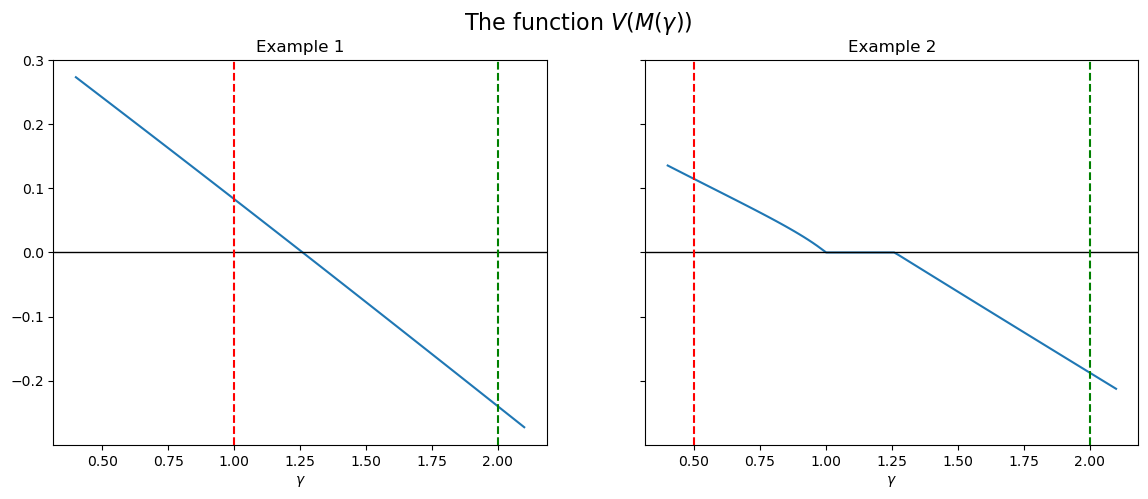
Furthermore, Hamburger et al. [Hamburger et al., 1967] show that the function \(\gamma \mapsto V(M(\gamma))\) is continuous and nonincreasing in \(\gamma\).
This suggests an algorithm to compute \((\alpha_0, x_0)\) and \((\beta_0, p_0)\) for a given input-output pair \((A, B)\).
37.5.2. Algorithm#
Hamburger, Thompson and Weil [Hamburger et al., 1967] propose a simple bisection algorithm to find the minimal and maximal roots (i.e. \(\beta_0\) and \(\alpha_0\)) of the function \(\gamma \mapsto V(M(\gamma))\).
37.5.2.1. Step 1#
First, notice that we can easily find trivial upper and lower bounds for \(\alpha_0\) and \(\beta_0\).
TEP requires that \(x^\top (B-\alpha A)\geq \mathbf{0}^\top\) and \(x > \mathbf{0}\), so if \(\alpha\) is so large that \(\max_i\{[(B-\alpha A)\iota_n]_i\} < 0\), then TEP ceases to have a solution.
Accordingly, let UB be the \(\alpha^{*}\) that
solves \(\max_i\{[(B-\alpha^{*} A)\iota_n]_i\} = 0\).
Similar to the upper bound, if \(\beta\) is so low that \(\min_j\{[\iota^\top_m(B-\beta A)]_j\}>0\), then the EEP has no solution and so we can define
LBas the \(\beta^{*}\) that solves \(\min_j\{[\iota^\top_m(B-\beta^{*} A)]_j\}=0\).
The bounds method calculates these trivial bounds for us
n1.bounds()
(1.0, 2.0)
37.5.2.2. Step 2#
Compute \(\alpha_0\) and \(\beta_0\)
Finding \(\alpha_0\)
Fix \(\gamma = \frac{UB + LB}{2}\) and compute the solution of the two-player zero-sum game associated with \(M(\gamma)\). We can use either the primal or the dual LP problem.
If \(V(M(\gamma)) \geq 0\), then set \(LB = \gamma\), otherwise let \(UB = \gamma\).
Iterate on 1. and 2. until \(|UB - LB| < \epsilon\).
Finding \(\beta_0\)
Fix \(\gamma = \frac{UB + LB}{2}\) and compute the solution of the two-player zero-sum game associated with \(M(\gamma)\). We can use either the primal or the dual LP problem.
If \(V(M(\gamma)) > 0\), then set \(LB = \gamma\), otherwise let \(UB = \gamma\).
Iterate on 1. and 2. until \(|UB - LB| < \epsilon\).
Existence: Since \(V(M(LB))>0\) and \(V(M(UB))<0\) and \(V(M(\cdot))\) is a continuous, nonincreasing function, there is at least one \(\gamma\in[LB, UB]\), s.t. \(V(M(\gamma))=0\).
The zerosum method calculates the value and optimal strategies associated with a given \(\gamma\).
γ = 2

print(f'Value of the game with γ = {γ}')
print(n1.zerosum(γ=γ)[0])
print('Intensity vector (from the primal)')
print(n1.zerosum(γ=γ)[1])
print('Price vector (from the dual)')
print(n1.zerosum(γ=γ, dual=True)[1])
Value of the game with γ = 2
-0.24
Intensity vector (from the primal)
[0.32 0.28 0.4 ]
Price vector (from the dual)
[0.4  0.32 0.28 0.  ]
numb_grid = 100
γ_grid = np.linspace(0.4, 2.1, numb_grid)

value_ex1_grid = np.asarray([n1.zerosum(γ=γ_grid[i])[0]
                            for i in range(numb_grid)])
value_ex2_grid = np.asarray([n2.zerosum(γ=γ_grid[i])[0]
                            for i in range(numb_grid)])

fig, axes = plt.subplots(1, 2, figsize=(14, 5), sharey=True)
fig.suptitle(r'The function $V(M(\gamma))$', fontsize=16)

for ax, grid, N, i in zip(axes, (value_ex1_grid, value_ex2_grid),
                          (n1, n2), (1, 2)):
    ax.plot(γ_grid, grid)
    ax.set(title=f'Example {i}', xlabel=r'$\gamma$')
    ax.axhline(0, c='k', lw=1)
    ax.axvline(N.bounds()[0], c='r', ls='--', label='lower bound')
    ax.axvline(N.bounds()[1], c='g', ls='--', label='upper bound')

plt.show()
The expansion method implements the bisection algorithm for \(\alpha_0\) (and uses the primal LP problem for \(x_0\))
α_0, x, p = n1.expansion()
print(f'α_0 = {α_0}')
print(f'x_0 = {x}')
print(f'The corresponding p from the dual = {p}')
α_0 = 1.2599210478365421
x_0 = [0.33 0.26 0.41]
The corresponding p from the dual = [0.41 0.33 0.26 0.  ]
The interest method implements the bisection algorithm for \(\beta_0\) (and uses the dual LP problem for \(p_0\))
β_0, x, p = n1.interest()
print(f'β_0 = {β_0}')
print(f'p_0 = {p}')
print(f'The corresponding x from the primal = {x}')
β_0 = 1.2599210478365421
p_0 = [0.41 0.33 0.26 0.  ]
The corresponding x from the primal = [0.33 0.26 0.41]
Of course, when \(\gamma^*\) is unique, it is irrelevant which one of the two methods we use – both work.
In particular, as will be shown below, in case of an irreducible \((A,B)\) (like in Example 1), the maximal and minimal roots of \(V(M(\gamma))\) necessarily coincide implying a ‘‘full duality’’ result, i.e. \(\alpha_0 = \beta_0 = \gamma^*\) so that the expansion (and interest) rate \(\gamma^*\) is unique.
37.5.3. Uniqueness and Irreducibility#
As an illustration, compute first the maximal and minimal roots of \(V(M(\cdot))\) for our Example 2 that has a reducible input-output pair \((A, B)\)
α_0, x, p = n2.expansion()
print(f'α_0 = {α_0}')
print(f'x_0 = {x}')
print(f'The corresponding p from the dual = {p}')
α_0 = 1.259921052493155
x_0 = [5.27e-10 0.00e+00 3.27e-01 2.60e-01 4.13e-01]
The corresponding p from the dual = [0.   0.21 0.33 0.26 0.21 0.  ]
β_0, x, p = n2.interest()
print(f'β_0 = {β_0}')
print(f'p_0 = {p}')
print(f'The corresponding x from the primal = {x}')
β_0 = 1.0000000009313226
p_0 = [ 5.00e-01  5.00e-01 -1.55e-09 -1.24e-09 -9.31e-10  0.00e+00]
The corresponding x from the primal = [-0.    0.    0.25  0.25  0.5 ]
As we can see, with a reducible \((A,B)\), the roots found by the bisection algorithms might differ, so there might be multiple \(\gamma^*\) that make the value of the game with \(M(\gamma^*)\) zero. (see the figure above).
Indeed, although the von Neumann theorem assures existence of the equilibrium, Assumption 37.1 and Assumption 37.2 are not sufficient for uniqueness. Nonetheless, Kemeny et al. (1967) show that there are at most finitely many economic solutions, meaning that there are only finitely many \(\gamma^*\) that satisfy \(V(M(\gamma^*)) = 0\) and \(x_0^\top Bp_0 > 0\) and that for each such \(\gamma^*_i\), there is a self-contained part of the economy (a sub-economy) that in equilibrium can expand independently with the expansion coefficient \(\gamma^*_i\).
The following theorem (see Theorem 9.10. in Gale [Gale, 1989]) asserts that imposing irreducibility is sufficient for uniqueness of \((\gamma^*, x_0, p_0)\).
Theorem 37.2
Adopt the conditions of Theorem 37.1. If the economy \((A,B)\) is irreducible, then \(\gamma^*=\alpha_0=\beta_0\).
37.5.4. A Special Case#
There is a special \((A,B)\) that allows us to simplify the solution method significantly by invoking the powerful Perron-Frobenius theorem for non-negative matrices.
Definition 37.5
We call an economy simple if it satisfies
\(n=m\)
Each activity produces exactly one good
Each good is produced by one and only one activity.
These assumptions imply that \(B=I_n\), i.e., that \(B\) can be written as an identity matrix (possibly after reshuffling its rows and columns).
The simple model has the following special property (Theorem 9.11. in Gale [Gale, 1989]): if \(x_0\) and \(\alpha_0>0\) solve the TEP with \((A,I_n)\), then
The latter shows that \(1/\alpha_0\) is a positive eigenvalue of \(A\) and \(x_0\) is the corresponding non-negative left eigenvector.
The classic result of Perron and Frobenius implies that a non-negative matrix has a non-negative eigenvalue-eigenvector pair.
Moreover, if \(A\) is irreducible, then the optimal intensity vector \(x_0\) is positive and unique up to multiplication by a positive scalar.
Suppose that \(A\) is reducible with \(k\) irreducible subsets \(S_1,\dots,S_k\). Let \(A_i\) be the submatrix corresponding to \(S_i\) and let \(\alpha_i\) and \(\beta_i\) be the associated expansion and interest factors, respectively. Then we have