63. Optimal Savings III: Stochastic Returns#
63.1. Overview#
In this lecture, we continue our study of optimal savings problems, building on Optimal Savings I: Cake Eating and Optimal Savings II: Numerical Cake Eating.
The key difference from the previous lectures is that wealth now evolves stochastically.
We can think of wealth as a harvest that regrows if we save some seeds.
Specifically, if we save and invest part of today’s harvest \(x_t\), it grows into next period’s harvest \(x_{t+1}\) according to a stochastic production process.
The extensions in this lecture introduce several new elements:
nonlinear returns to saving, through a production function, and
stochastic returns, due to shocks to production.
Despite these additions, the model remains relatively tractable.
As a first pass, we will solve the model using dynamic programming and value function iteration (VFI).
Note
In later lectures we’ll explore more efficient methods for this class of problems.
At the same time, VFI is foundational and globally convergent.
Hence we want to be sure we can use this method too.
More information on this savings problem can be found in
[Ljungqvist and Sargent, 2018], Section 3.1
EDTC, Chapter 1
[Sundaram, 1996], Chapter 12
Let’s start with some imports:
import matplotlib.pyplot as plt
import numpy as np
from scipy.interpolate import interp1d
from scipy.optimize import minimize_scalar
from typing import NamedTuple, Callable
63.2. The Model#
Here we described the new model and the optimization problem.
63.2.1. Setup#
Consider an agent who owns an amount \(x_t \in \mathbb R_+ := [0, \infty)\) of a consumption good at time \(t\).
This output can either be consumed or saved and used for production.
Production is stochastic, in that it also depends on a shock \(\xi_{t+1}\) realized at the end of the current period.
Next period output is
where \(f \colon \mathbb R_+ \to \mathbb R_+\) is the production function and
is current savings.
and all variables are required to be nonnegative.
In what follows,
The sequence \(\{\xi_t\}\) is assumed to be IID.
The common distribution of each \(\xi_t\) will be denoted by \(\phi\).
The production function \(f\) is assumed to be increasing and continuous.
63.2.2. Optimization#
Taking \(x_0\) as given, the agent wishes to maximize
subject to
where
\(u\) is a bounded, continuous and strictly increasing utility function and
\(\beta \in (0, 1)\) is a discount factor.
In summary, the agent’s aim is to select a path \(c_0, c_1, c_2, \ldots\) for consumption that is
nonnegative,
feasible,
optimal, in the sense that it maximizes (63.2) relative to all other feasible consumption sequences, and
adapted, in the sense that the current action \(c_t\) depends only on current and historical outcomes, not on future outcomes such as \(\xi_{t+1}\).
In the present context
\(x_t\) is called the state variable — it summarizes the “state of the world” at the start of each period.
\(c_t\) is called the control variable — a value chosen by the agent each period after observing the state.
63.2.3. Optimal Policies#
Let us look at policy functions, each one of which is a map \(\sigma\) from the current state \(x_t\) into a current action \(c_t\).
Note
These kinds of policies are called Markov policies (or stationary Markov policies).
For this dynamic program, the optimal policy is always a Markov policy (see, e.g., DP1).
In essence, the current state \(x_t\) provides a sufficient statistic for the history in terms of making an optimal decision today.
In what follows, we will call \(\sigma\) a feasible consumption policy if it satisfies
In other words, a feasible policy is a policy function that respects the resource constraint.
The set of all feasible consumption policies will be denoted by \(\Sigma\).
Each \(\sigma \in \Sigma\) determines a Markov dynamics for output \(\{x_t\}\) via
This is the time path for output when we choose and stick with the policy \(\sigma\).
We insert this process into the objective function to get
This is the total expected present value of following policy \(\sigma\) forever, given initial income \(x_0\).
The aim is to select a policy that makes this number as large as possible.
The next section covers these ideas more formally.
63.2.4. Optimality#
The lifetime value \(v_{\sigma}\) associated with a given policy \(\sigma\) is the mapping defined by
when \(\{x_t\}\) is given by (63.5) with \(x_0 = x\).
In other words, it is the lifetime value of following policy \(\sigma\) forever, starting at initial condition \(x\).
The value function is then defined as
The value function gives the maximal value that can be obtained from state \(x\), after considering all feasible policies.
A policy \(\sigma \in \Sigma\) is called optimal if \(v_\sigma(x) = v^*(x)\) for all \(x \in \mathbb R_+\).
63.2.5. The Bellman Equation#
The following equation is called the Bellman equation associated with this dynamic programming problem.
This is a functional equation in \(v\), in the sense that a given \(v\) can either satisfy it or not satisfy it.
The term \(\int v(f(x - c) z) \phi(dz)\) can be understood as the expected next period value when
\(v\) is used to measure value
the state is \(x\)
consumption is set to \(c\)
As shown in DP1 and a range of other texts, the value function \(v^*\) satisfies the Bellman equation.
In other words, (63.9) holds when \(v=v^*\).
The intuition is that maximal value from a given state can be obtained by optimally trading off
current reward from a given action, vs
expected discounted future value of the state resulting from that action
The Bellman equation is important because it
gives us more information about the value function and
suggests a way of computing the value function, which we discuss below.
63.2.6. Greedy Policies#
The value function can be used to compute optimal policies.
Given a continuous function \(v\) on \(\mathbb R_+\), we say that \(\sigma \in \Sigma\) is \(v\)-greedy if
for every \(x \in \mathbb R_+\).
In other words, \(\sigma \in \Sigma\) is \(v\)-greedy if it optimally trades off current and future rewards when \(v\) is taken to be the value function.
In our setting, we have the following key result
Theorem 63.1
A feasible consumption policy is optimal if and only if it is \(v^*\)-greedy.
See, for example, Theorem 10.1.11 of EDTC.
Hence, once we have a good approximation to \(v^*\), we can compute the (approximately) optimal policy by computing the corresponding greedy policy.
The advantage is that we are now solving a much lower dimensional optimization problem.
63.2.7. The Bellman Operator#
How, then, should we compute the value function?
One way is to use the so-called Bellman operator.
(The term operator is usually reserved for functions that send functions into functions!)
The Bellman operator is denoted by \(T\) and defined by
In other words, \(T\) sends the function \(v\) into the new function \(Tv\) defined by (63.11).
By construction, the set of solutions to the Bellman equation (63.9) exactly coincides with the set of fixed points of \(T\).
For example, if \(Tv = v\), then, for any \(x \geq 0\),
which says precisely that \(v\) is a solution to the Bellman equation.
It follows that \(v^*\) is a fixed point of \(T\).
63.2.8. Review of Theoretical Results#
One can also show that \(T\) is a contraction mapping on the set of continuous bounded functions on \(\mathbb R_+\) under the supremum distance
See EDTC, Lemma 10.1.18.
Hence, it has exactly one fixed point in this set, which we know is equal to the value function.
It follows that
The value function \(v^*\) is bounded and continuous.
Starting from any bounded and continuous \(v\), the sequence \(v, Tv, T^2v, \ldots\) generated by iteratively applying \(T\) converges uniformly to \(v^*\).
This iterative method is called value function iteration.
We also know that a feasible policy is optimal if and only if it is \(v^*\)-greedy.
It’s not too hard to show that a \(v^*\)-greedy policy exists.
Hence, at least one optimal policy exists.
Our problem now is how to compute it.
63.2.9. Unbounded Utility#
The results stated above assume that \(u\) is bounded.
In practice economists often work with unbounded utility functions — and so will we.
In the unbounded setting, various optimality theories exist.
Nevertheless, their main conclusions are usually in line with those stated for the bounded case just above (as long as we drop the word “bounded”).
Note
Consult the following references for more on the unbounded case:
The lecture The Income Fluctuation Problem V: Stochastic Returns on Assets.
Section 12.2 of EDTC.
63.3. Computation#
Let’s now look at computing the value function and the optimal policy.
Our implementation in this lecture will focus on clarity and flexibility.
(In subsequent lectures we will focus on efficiency and speed.)
We will use fitted value function iteration, which was already described in Optimal Savings II: Numerical Cake Eating.
63.3.1. Scalar Maximization#
To maximize the right hand side of the Bellman equation (63.9), we are going to use
the minimize_scalar routine from SciPy.
To keep the interface tidy, we will wrap minimize_scalar in an outer function as follows:
def maximize(g, upper_bound):
    """
    Maximize the function g over the interval [0, upper_bound].

    We use the fact that the maximizer of g on any interval is
    also the minimizer of -g.

    """

    objective = lambda x: -g(x)
    bounds = (0, upper_bound)
    result = minimize_scalar(objective, bounds=bounds, method='bounded')
    maximizer, maximum = result.x, -result.fun
    return maximizer, maximum
63.3.2. Model#
We will assume for now that \(\phi\) is the distribution of \(\xi := \exp(\mu + \nu \zeta)\) where
\(\zeta\) is standard normal,
\(\mu\) is a shock location parameter and
\(\nu\) is a shock scale parameter.
We will store the primitives of the model in a NamedTuple.
class Model(NamedTuple):
    u: Callable        # utility function
    f: Callable        # production function
    β: float           # discount factor
    μ: float           # shock location parameter
    ν: float           # shock scale parameter
    x_grid: np.ndarray # state grid
    shocks: np.ndarray # shock draws


def create_model(
        u: Callable,
        f: Callable,
        β: float = 0.96,
        μ: float = 0.0,
        ν: float = 0.1,
        grid_max: float = 4.0,
        grid_size: int = 120,
        shock_size: int = 250,
        seed: int = 1234
    ) -> Model:
    """
    Creates an instance of the optimal savings model.
    """
    # Set up grid
    x_grid = np.linspace(1e-4, grid_max, grid_size)

    # Store shocks (with a seed, so results are reproducible)
    np.random.seed(seed)
    shocks = np.exp(μ + ν * np.random.randn(shock_size))

    return Model(u, f, β, μ, ν, x_grid, shocks)
We set up the right-hand side of the Bellman equation
def B(
        x: float,              # State
        c: float,              # Action
        v_array: np.ndarray,   # Array representing a guess of the value fn
        model: Model           # An instance of Model containing parameters
    ):

    u, f, β, μ, ν, x_grid, shocks = model
    v = interp1d(x_grid, v_array)

    return u(c) + β * np.mean(v(f(x - c) * shocks))
In the second last line we are using linear interpolation.
In the last line, the expectation in (63.11) is computed via Monte Carlo, using the approximation
where \(\{\xi_i\}_{i=1}^n\) are IID draws from \(\phi\).
Monte Carlo is not always the most efficient way to compute integrals numerically but it does have some theoretical advantages in the present setting.
(For example, it preserves the contraction mapping property of the Bellman operator — see, e.g., [Pál and Stachurski, 2013].)
63.3.3. The Bellman Operator#
The next function implements the Bellman operator.
def T(v: np.ndarray, model: Model) -> tuple[np.ndarray, np.ndarray]:
    """
    The Bellman operator.  Updates the guess of the value function.

      * model is an instance of Model
      * v is an array representing a guess of the value function

    """
    x_grid = model.x_grid
    v_new = np.empty_like(v)

    for i in range(len(x_grid)):
        x = x_grid[i]
        _, v_max = maximize(lambda c: B(x, c, v, model), x)
        v_new[i] = v_max

    return v_new
Here’s the function:
def get_greedy(
        v: np.ndarray,          # current guess of the value function
        model: Model            # instance of optimal savings model
    ):
    " Compute the v-greedy policy on x_grid."

    σ = np.empty_like(v)

    for i, x in enumerate(model.x_grid):
        # Maximize RHS of Bellman equation at state x
        σ[i], _ = maximize(lambda c: B(x, c, v, model), x)

    return σ
63.3.4. An Example#
Let’s suppose now that
For this particular problem, an exact analytical solution is available (see [Ljungqvist and Sargent, 2018], section 3.1.2), with
and optimal consumption policy
It is valuable to have these closed-form solutions because it lets us check whether our code works for this particular case.
In Python, the functions above can be expressed as:
def v_star(x, α, β, μ):
    """
    True value function
    """
    c1 = np.log(1 - α * β) / (1 - β)
    c2 = (μ + α * np.log(α * β)) / (1 - α)
    c3 = 1 / (1 - β)
    c4 = 1 / (1 - α * β)
    return c1 + c2 * (c3 - c4) + c4 * np.log(x)

def σ_star(x, α, β):
    """
    True optimal policy
    """
    return (1 - α * β) * x
Next let’s create an instance of the model with the above primitives and assign it to the variable model.
α = 0.4
def fcd(s):
    return s**α

model = create_model(u=np.log, f=fcd)
Now let’s see what happens when we apply our Bellman operator to the exact solution \(v^*\) in this case.
In theory, since \(v^*\) is a fixed point, the resulting function should again be \(v^*\).
In practice, we expect some small numerical error.
x_grid = model.x_grid

v_init = v_star(x_grid, α, model.β, model.μ)    # Start at the solution
v = T(v_init, model)             # Apply T once

fig, ax = plt.subplots()
ax.set_ylim(-35, -24)
ax.plot(x_grid, v, lw=2, alpha=0.6, label='$Tv^*$')
ax.plot(x_grid, v_init, lw=2, alpha=0.6, label='$v^*$')
ax.legend()
plt.show()
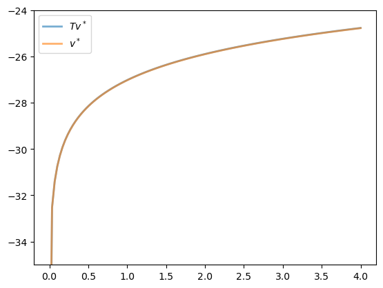
The two functions are essentially indistinguishable, so we are off to a good start.
Now let’s have a look at iterating with the Bellman operator, starting from an arbitrary initial condition.
The initial condition we’ll start with is, somewhat arbitrarily, \(v(x) = 5 \ln (x)\).
v = 5 * np.log(x_grid)  # An initial condition
n = 35

fig, ax = plt.subplots()

ax.plot(x_grid, v, color=plt.cm.jet(0),
        lw=2, alpha=0.6, label='Initial condition')

for i in range(n):
    v = T(v, model)  # Apply the Bellman operator
    ax.plot(x_grid, v, color=plt.cm.jet(i / n), lw=2, alpha=0.6)

ax.plot(x_grid, v_star(x_grid, α, model.β, model.μ), 'k-', lw=2,
        alpha=0.8, label='True value function')

ax.legend()
ax.set(ylim=(-40, 10), xlim=(np.min(x_grid), np.max(x_grid)))
plt.show()
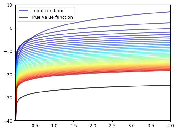
The figure shows
the first 36 functions generated by the fitted value function iteration algorithm, with hotter colors given to higher iterates
the true value function \(v^*\) drawn in black
The sequence of iterates converges towards \(v^*\).
We are clearly getting closer.
63.3.5. Iterating to Convergence#
We can write a function that iterates until the difference is below a particular tolerance level.
def solve_model(
        model: Model,           # instance of optimal savings model
        tol: float = 1e-4,      # convergence tolerance
        max_iter: int = 1000,   # maximum iterations
        verbose: bool = True,   # print iteration info
        print_skip: int = 25    # iterations between prints
    ):
    " Solve by value function iteration. "

    v = model.u(model.x_grid)  # Initial condition
    i = 0
    error = tol + 1

    while i < max_iter and error > tol:
        v_new = T(v, model)
        error = np.max(np.abs(v - v_new))
        i += 1
        if verbose and i % print_skip == 0:
            print(f"Error at iteration {i} is {error}.")
        v = v_new

    if error > tol:
        print("Failed to converge!")
    elif verbose:
        print(f"\nConverged in {i} iterations.")

    v_greedy = get_greedy(v_new, model)
    return v_greedy, v_new
Let’s use this function to compute an approximate solution at the defaults.
v_greedy, v_solution = solve_model(model)
Error at iteration 25 is 0.40975776844490497.
Error at iteration 50 is 0.1476753540823772.
Error at iteration 75 is 0.05322171277213883.
Error at iteration 100 is 0.019180930548646558.
Error at iteration 125 is 0.006912744396021964.
Error at iteration 150 is 0.0024913303848137502.
Error at iteration 175 is 0.0008978672913073638.
Error at iteration 200 is 0.00032358842396718046.
Error at iteration 225 is 0.00011662020561686859.

Converged in 229 iterations.
Now we check our result by plotting it against the true value:
fig, ax = plt.subplots()

ax.plot(x_grid, v_solution, lw=2, alpha=0.6,
        label='Approximate value function')

ax.plot(x_grid, v_star(x_grid, α, model.β, model.μ), lw=2,
        alpha=0.6, label='True value function')

ax.legend()
ax.set_ylim(-35, -24)
plt.show()
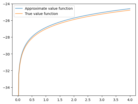
The figure shows that we are pretty much on the money.
63.3.6. The Policy Function#
The policy v_greedy computed above corresponds to an approximate optimal policy.
The next figure compares it to the exact solution, which, as mentioned above, is \(\sigma(x) = (1 - \alpha \beta) x\)
fig, ax = plt.subplots()

ax.plot(x_grid, v_greedy, lw=2,
        alpha=0.6, label='approximate policy function')

ax.plot(x_grid, σ_star(x_grid, α, model.β), '--',
        lw=2, alpha=0.6, label='true policy function')

ax.legend()
plt.show()
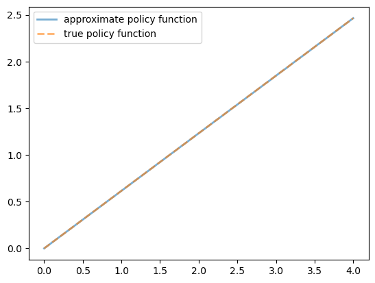
The figure shows that we’ve done a good job in this instance of approximating the true policy.
63.4. Exercises#
Exercise 63.1
A common choice for utility function in this kind of work is the CRRA specification
Maintaining the other defaults, including the Cobb-Douglas production function, solve the optimal savings model with this utility specification.
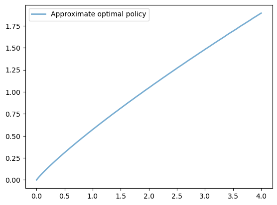
Setting \(\gamma = 1.5\), compute and plot an estimate of the optimal policy.
Solution
Here we set up the model.
γ = 1.5   # Preference parameter

def u_crra(c):
    return (c**(1 - γ) - 1) / (1 - γ)

model = create_model(u=u_crra, f=fcd)
Now let’s run it, with a timer.
%%time
v_greedy, v_solution = solve_model(model)
Error at iteration 25 is 0.5528151810315194.
Error at iteration 50 is 0.19923228425591333.
Error at iteration 75 is 0.07180266113797629.
Error at iteration 100 is 0.025877443335843964.
Error at iteration 125 is 0.009326145618956616.
Error at iteration 150 is 0.003361112262041388.
Error at iteration 175 is 0.0012113338242443206.
Error at iteration 200 is 0.0004365607333056687.
Error at iteration 225 is 0.00015733505506432266.

Converged in 237 iterations.
CPU times: user 27 s, sys: 4.01 ms, total: 27 s
Wall time: 27 s
Let’s plot the policy function just to see what it looks like:
fig, ax = plt.subplots()
ax.plot(x_grid, v_greedy, lw=2,
        alpha=0.6, label='Approximate optimal policy')
ax.legend()
plt.show()