87. Two-Country Model with Distorting Taxes#
87.1. Overview#
This lecture is a sequel to this QuantEcon lecture Cass-Koopmans Model with Distorting Taxes in which we studied consequences of foreseen fiscal and technology shocks on competitive equilibrium prices and quantities in a nonstochastic version of a Cass-Koopmans growth model like the one described in this QuantEcon lecture Cass-Koopmans Competitive Equilibrium.
Here we study a two-country version of that model.
We construct it by putting instances of two Cass-Koopmans Competitive Equilibrium economies together back to back, and then opening international trade in some commodities, but not in others.
This lets us focus on some of the issues studied by Mendoza and Tesar [1998].
Let’s start with some imports:
import numpy as np
from scipy.optimize import root
import matplotlib.pyplot as plt
from collections import namedtuple
from mpmath import mp, mpf
from warnings import warn

# Set the precision
mp.dps = 40
mp.pretty = True
87.2. A Two-Country Cass-Koopmans Model#
This section describes a two-country version of the basic model of The Economy.
The model has a structure similar to ones used in the international real business cycle literature and is in the spirit of an analysis of distorting taxes by Mendoza and Tesar [1998].
We allow two countries to trade goods and claims on future goods, but not labor.
Both countries have production technologies, and consumers in each country can hold capital in either country, subject to different tax treatments.
We denote variables in the second country with asterisks (*).
Households in both countries maximize lifetime utility:
where \(u(c) = \frac{c^{1-\gamma}}{1-\gamma}\) with \(\gamma > 0\).
There are Cobb-Douglas functions with identical technology parameters in the two countries.
The world resource constraint in this two-country economy is:
which combines the feasibility constraints for the two countries.
Later, we will use this constraint as a global feasibility constraint in our computation.
To connect the two countries, we need to specify how capital flows across borders and how taxes are levied in different jurisdictions.
87.2.1. Capital Mobility and Taxation#
A consumer in country one can hold capital in either country but pays taxes on rentals from foreign holdings of capital at the rate set by the foreign country.
Residents in both countries can purchase consumption at date \(t\) at a common Arrow-Debreu price \(q_t\). We assume capital markets are complete.
Let \(B_t^f\) be the amount of time \(t\) goods that the representative domestic consumer raises by issuing a one-period IOU to the representative foreign consumer.
So \(B_t^f > 0\) indicates the domestic consumer is borrowing from abroad at \(t\), and \(B_t^f < 0\) indicates the domestic consumer is lending abroad at \(t\).
Hence, the budget constraint of a representative consumer in country one is:
No-arbitrage conditions for \(k_t\) and \(\tilde{k}_t\) for \(t \geq 1\) imply
which together imply that after-tax rental rates on capital are equalized across the two countries:
The no-arbitrage conditions for \(B_t^f\) for \(t \geq 0\) are \(q_t = q_{t+1} R_{t+1,t}\), which implies that
for \(t \geq 1\).
Since domestic capital, foreign capital, and consumption loans bear the same rates of return, portfolios are indeterminate.
We can set holdings of foreign capital equal to zero in each country if we allow \(B_t^f\) to be nonzero.
This way of resolving portfolio indeterminacy is convenient because it reduces the number of initial conditions we need to specify.
Therefore, we set holdings of foreign capital equal to zero in both countries while allowing international lending.
Given an initial level \(B_{-1}^f\) of debt from the domestic country to the foreign country, and where \(R_{t-1,t} = \frac{q_{t-1}}{q_t}\), international debt dynamics satisfy
def Bf_path(k, c, g, model):
    """
    Compute B^{f}_t:
      Bf_t = R_{t-1} Bf_{t-1} + c_t + (k_{t+1}-(1-δ)k_t) + g_t - f(k_t)
    with Bf_0 = 0.
    """
    S = len(c) - 1
    R = c[:-1]**(-model.γ) / (model.β * c[1:]**(-model.γ))

    Bf = np.zeros(S + 1)
    for t in range(1, S + 1):
        inv = k[t] - (1 - model.δ) * k[t-1]
        Bf[t] = (
            R[t-1] * Bf[t-1] + c[t] + inv + g[t-1]
            - f(k[t-1], model))
    return Bf

def Bf_ss(c_ss, k_ss, g_ss, model):
    """
    Compute the steady-state B^f
    """
    R_ss   = 1.0 / model.β
    inv_ss = model.δ * k_ss
    num    = c_ss + inv_ss + g_ss - f(k_ss, model)
    den    = 1.0 - R_ss
    return num / den
and
The firms’ first-order conditions in the two countries are:
International trade in goods establishes:
where \(\mu^*\) is a nonnegative number that is a function of the Lagrange multiplier on the budget constraint for a consumer in country \(*\).
We have normalized the Lagrange multiplier on the budget constraint of the domestic country to set the corresponding \(\mu\) for the domestic country to unity.
def compute_rs(c_t, c_tp1, c_s_t, c_s_tp1, τc_t,
               τc_tp1, τc_s_t, τc_s_tp1, model):
    """
    Compute international risk sharing after trade starts.
    """

    return (c_t**(-model.γ)/(1+τc_t)) * ((1+τc_s_t)/c_s_t**(-model.γ)) - (
        c_tp1**(-model.γ)/(1+τc_tp1)) * ((1+τc_s_tp1)/c_s_tp1**(-model.γ))
Equilibrium requires that the following two national Euler equations be satisfied for \(t \geq 0\):
The following code computes both the domestic and foreign Euler equations.
Since they have the same form but use different variables, we can write a single function that handles both cases.
def compute_euler(c_t, c_tp1, τc_t,
                    τc_tp1, τk_tp1, k_tp1, model):
    """
    Compute the Euler equation.
    """
    Rbar = (1 - τk_tp1)*(f_prime(k_tp1, model) - model.δ) + 1
    return model.β * (c_tp1/c_t)**(-model.γ) * (1+τc_t)/(1+τc_tp1) * Rbar - 1
87.2.2. Initial condition and steady state#
For the initial conditions, we choose the pre-trade allocation of capital (\(k_0, k_0^*\)) and the initial level \(B_{-1}^f\) of international debt owed by the unstarred (domestic) country to the starred (foreign) country.
87.2.3. Equilibrium steady state values#
The steady state of the two-country model is characterized by two sets of equations.
First, the following equations determine the steady-state capital-labor ratios \(\bar k\) and \(\bar k^*\) in each country:
Given these steady-state capital-labor ratios, the domestic and foreign consumption values \(\bar c\) and \(\bar c^*\) are determined by:
Equation (87.3) expresses feasibility at the steady state, while equation (87.4) represents the trade balance, including interest payments, at the steady state.
The steady-state level of debt \(\bar{B}^f\) from the domestic country to the foreign country influences the consumption allocation between countries but not the total world capital stock.
We assume \(\bar{B}^f = 0\) in the steady state, which gives us the following function to compute the steady-state values of capital and consumption
def compute_steady_state_global(model, g_ss=0.2):
    """
    Calculate steady state values for capital, consumption, and investment.
    """
    k_ss = ((1/model.β - (1-model.δ)) / (model.A * model.α)) ** (1/(model.α-1))
    c_ss = f(k_ss, model) - model.δ * k_ss - g_ss
    return k_ss, c_ss
Now, we can apply the residual minimization method to compute the steady-state values of capital and consumption.
Again, we minimize the residuals of the Euler equation, the global resource constraint, and the no-arbitrage condition.
def compute_residuals_global(z, model, shocks, T, k0_ss, k_star, Bf_star):
    """
    Compute residuals for the two-country model.
    """
    k, c, k_s, c_s = z.reshape(T+1, 4).T
    g, gs = shocks['g'], shocks['g_s']
    τc, τk = shocks['τ_c'], shocks['τ_k']
    τc_s, τk_s = shocks['τ_c_s'], shocks['τ_k_s']

    res = [k[0] - k0_ss, k_s[0] - k0_ss]

    for t in range(T):
        e_d = compute_euler(
            c[t], c[t+1],
            τc[t], τc[t+1], τk[t+1],
            k[t+1], model)

        e_f = compute_euler(
            c_s[t], c_s[t+1],
            τc_s[t], τc_s[t+1], τk_s[t+1],
            k_s[t+1], model)

        rs = compute_rs(
            c[t], c[t+1], c_s[t], c_s[t+1],
            τc[t], τc[t+1], τc_s[t], τc_s[t+1],
            model)

        # Global resource constraint
        grc = k[t+1] + k_s[t+1] - (
            f(k[t], model) + f(k_s[t], model) +
            (1-model.δ)*(k[t] + k_s[t]) -
            c[t] - c_s[t] - g[t] - gs[t]
        )

        res.extend([e_d, e_f, rs, grc])

    Bf_term = Bf_path(k, c, shocks['g'], model)[-1]
    res.append(k[T] - k_star)
    res.append(Bf_term - Bf_star)
    return np.array(res)
Now we plot the results
# Function to plot global two-country model results
def plot_global_results(k, k_s, c, c_s, shocks, model,
                        k0_ss, c0_ss, g_ss, S, T=40, shock='g',
                        # a dictionary storing sequence for lower left panel
                        ll_series='None'):
    """
    Plot results for the two-country model.
    """
    fig, axes = plt.subplots(2, 3, figsize=(10, 8))
    x = np.arange(T)
    τc, τk = shocks['τ_c'], shocks['τ_k']
    Bf = Bf_path(k, c, shocks['g'], model)

    # Compute derived series
    R_ratio = c[:-1]**(-model.γ) / (model.β * c[1:]**(-model.γ)) \
    *(1+τc[:-1])/(1+τc[1:])
    inv = k[1:] - (1-model.δ)*k[:-1]
    inv_s = k_s[1:] - (1-model.δ)*k_s[:-1]

    # Add initial conditions into the series
    R_ratio = np.append(1/model.β, R_ratio)
    c = np.append(c0_ss, c)
    c_s = np.append(c0_ss, c_s)
    k = np.append(k0_ss, k)
    k_s = np.append(k0_ss, k_s)

    # Capital
    axes[0,0].plot(x, k[:T], '-', lw=1.5)
    axes[0,0].plot(x, np.full(T, k0_ss), 'k-.', lw=1.5)
    axes[0,0].plot(x, k_s[:T], '--', lw=1.5)
    axes[0,0].set_title('k')
    axes[0,0].set_xlim(0, T-1)

    # Consumption
    axes[0,1].plot(x, c[:T], '-', lw=1.5)
    axes[0,1].plot(x, np.full(T, c0_ss), 'k-.', lw=1.5)
    axes[0,1].plot(x, c_s[:T], '--', lw=1.5)
    axes[0,1].set_title('c')
    axes[0,1].set_xlim(0, T-1)

    # Interest rate
    axes[0,2].plot(x, R_ratio[:T], '-', lw=1.5)
    axes[0,2].plot(x, np.full(T, 1/model.β), 'k-.', lw=1.5)
    axes[0,2].set_title(r'$\bar{R}$')
    axes[0,2].set_xlim(0, T-1)

    # Investment
    axes[1,0].plot(x, np.full(T, model.δ * k0_ss),
    'k-.', lw=1.5)
    axes[1,0].plot(x, np.append(model.δ*k0_ss, inv[:T-1]),
    '-', lw=1.5)
    axes[1,0].plot(x, np.append(model.δ*k0_ss, inv_s[:T-1]),
    '--', lw=1.5)
    axes[1,0].set_title('x')
    axes[1,0].set_xlim(0, T-1)

    # Shock
    axes[1,1].plot(x, shocks[shock][:T], '-', lw=1.5)
    axes[1,1].plot(x, np.full(T, shocks[shock][0]), 'k-.', lw=1.5)
    axes[1,1].set_title(f'${shock}$')
    axes[1,1].set_ylim(-0.1, 0.5)
    axes[1,1].set_xlim(0, T-1)

    # Capital flow
    axes[1,2].plot(x, np.append(0, Bf[1:T]), lw=1.5)
    axes[1,2].plot(x, np.zeros(T), 'k-.', lw=1.5)
    axes[1,2].set_title(r'$B^{f}$')
    axes[1,2].set_xlim(0, T-1)

    plt.tight_layout()
    return fig, axes
As in our in the one-country model in Cass-Koopmans Model with Distorting Taxes, we assume a Cobb-Douglas production function:
def f(k, model, A=1):
    """
    Production function: f(k) = A * k^{α}
    """
    return A * k ** model.α

def f_prime(k, model, A=1):
    """
    Marginal product of capital: f'(k) = α * A * k^{α - 1}
    """
    return model.α * A * k ** (model.α - 1)
Similarly, we define the capital rental rate
def compute_η_path(k_path, model, S=100, A_path=None):
    """
    Compute η path: η_t = f'(k_t)
    with optional A_path for growth models.
    """
    A = np.ones_like(k_path) if A_path is None else np.asarray(A_path)
    η_path = np.zeros_like(k_path)
    for t in range(S):
        η_path[t] = f_prime(k_path[t], model, A[t])
    return η_path
87.2.3.1. Experiment 1: A foreseen increase in \(g\) from 0.2 to 0.4 at t=10#
The figure below presents transition dynamics after an increase in \(g\) in the domestic economy from 0.2 to 0.4 that is announced ten periods in advance.
We start both economies from a steady state with \(B_0^f = 0\).
In the figure below, the blue lines represent the domestic economy and orange dotted lines represent the foreign economy.
Model = namedtuple("Model", ["β", "γ", "δ", "α", "A"])
model = Model(β=0.95, γ=2.0, δ=0.2, α=0.33, A=1.0)
S = 100

shocks_global = {
    'g': np.concatenate((np.full(10, 0.2), np.full(S-9, 0.4))),
    'g_s': np.full(S+1, 0.2),
    'τ_c': np.zeros(S+1),
    'τ_k': np.zeros(S+1),
    'τ_c_s': np.zeros(S+1),
    'τ_k_s': np.zeros(S+1)
}
g_ss = 0.2
k0_ss, c0_ss = compute_steady_state_global(model, g_ss)

k_star = k0_ss
Bf_star = Bf_ss(c0_ss, k_star, g_ss, model)

init_glob = np.tile([k0_ss, c0_ss, k0_ss, c0_ss], S+1)
sol_glob = root(
    lambda z: compute_residuals_global(z, model, shocks_global,
                                        S, k0_ss, k_star, Bf_star),
    init_glob, tol=1e-12
)
k, c, k_s, c_s = sol_glob.x.reshape(S+1, 4).T

# Plot global results via function
plot_global_results(k, k_s, c, c_s,
                        shocks_global, model,
                        k0_ss, c0_ss, g_ss,
                        S)
plt.show()
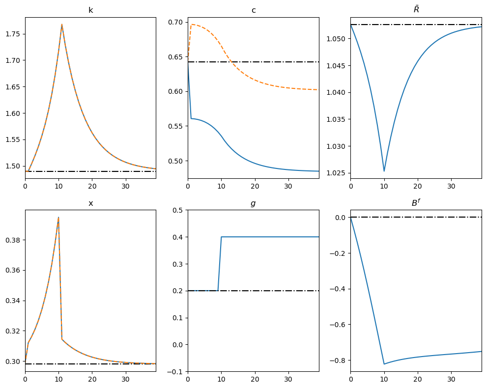
At time 1, the government announces that domestic government purchases \(g\) will rise ten periods later, cutting into future private resources.
To smooth consumption, domestic households immediately increase saving, offsetting the anticipated hit to their future wealth.
In a closed economy, they would save solely by accumulating extra domestic capital; with open capital markets, they can also lend to foreigners.
Once the capital flow opens up at time \(1\), the no-arbitrage conditions connect adjustments of both types of saving: the increase in savings by domestic households will reduce the equilibrium return on bonds and capital in the foreign economy to prevent arbitrage opportunities.
Because no-arbitrage equalizes the ratio of marginal utilities, the resulting paths of consumption and capital are synchronized across the two economies.
Up to the date the higher \(g\) takes effect, both countries continue to build their capital stocks.
When government spending finally rises 10 periods later, domestic households begin to draw down part of that capital to cushion consumption.
Again by no-arbitrage conditions, when \(g\) actually increases, both countries reduce their investment rates.
The domestic economy, in turn, starts running current-account deficits partially to fund the increase in \(g\).
This means that foreign households begin repaying part of their external debt by reducing their capital stock.
87.2.3.2. Experiment 2: A foreseen increase in \(g\) from 0.2 to 0.4 at t=10#
We now explore the impact of an increase in capital taxation in the domestic economy \(10\) periods after its announcement at \(t = 1\).
Because the change is anticipated, households in both countries adjust immediately–even though the tax does not take effect until period \(t = 11\).
shocks_global = {
    'g': np.full(S+1, g_ss),
    'g_s': np.full(S+1, g_ss),
    'τ_c': np.zeros(S+1),
    'τ_k': np.concatenate((np.zeros(10), np.full(S-9, 0.2))),
    'τ_c_s': np.zeros(S+1),
    'τ_k_s': np.zeros(S+1),
}

k0_ss, c0_ss = compute_steady_state_global(model, g_ss)
k_star = k0_ss
Bf_star = Bf_ss(c0_ss, k_star, g_ss, model)

init_glob = np.tile([k0_ss, c0_ss, k0_ss, c0_ss], S+1)

sol_glob = root(
    lambda z: compute_residuals_global(z, model,
            shocks_global, S, k0_ss, k_star, Bf_star),
            init_glob, tol=1e-12)

k, c, k_s, c_s = sol_glob.x.reshape(S+1, 4).T

# plot
fig, axes = plot_global_results(k, k_s, c, c_s, shocks_global, model,
                                k0_ss, c0_ss, g_ss, S, shock='τ_k')
plt.tight_layout()
plt.show()
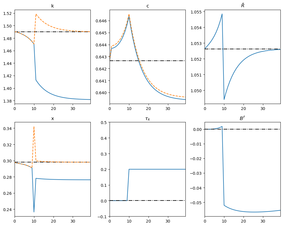
After the tax increase is announced, domestic households foresee lower after-tax returns on capital, so they shift toward higher present consumption and allow the domestic capital stock to decline.
This shrinkage of the world capital supply drives the global real interest rate upward, prompting foreign households to raise current consumption as well.
Prior to the actual tax hike, the domestic economy finances part of its consumption by importing capital, generating a current-account deficit.
When \(\tau_k\) finally rises, international arbitrage leads investors to reallocate capital quickly toward the untaxed foreign market, compressing the yield on bonds everywhere.
The bond-rate drop reflects the lower after-tax return on domestic capital and the higher foreign capital stock, which depresses its marginal product.
Foreign households fund their capital purchases by borrowing abroad, creating a pronounced current-account deficit and a buildup of external debt.
After the policy change, both countries move smoothly toward a new steady state in which:
Consumption levels in each economy settle below their pre-announcement paths.
Capital stocks differ just enough to equalize after-tax returns across borders.
Despite carrying positive net liabilities, the foreign country enjoys higher steady-state consumption because its larger capital stock yields greater output.
The episode demonstrates how open capital markets transmit a domestic tax shock internationally: capital flows and interest-rate movements share the burden, smoothing consumption adjustments in both the taxed and untaxed economies over time.
Exercise 87.1
In this exercise, replace the plot for \({x_t}\) with \(\eta_t\) to replicate the figure in [Ljungqvist and Sargent, 2018].
Compare the figures for \({k_t}\) and \(\eta_t\) and discuss the economic intuition.
Solution
Here is one solution.
fig, axes = plot_global_results(k, k_s, c, c_s, shocks_global, model,
                                k0_ss, c0_ss, g_ss, S, shock='τ_k')

# Clear the plot for x_t
axes[1,0].cla()

# Plot η_t
axes[1,0].plot(compute_η_path(k, model)[:40])
axes[1,0].plot(compute_η_path(k_s, model)[:40], '--')
axes[1,0].plot(np.full(40, f_prime(k_s, model)[0]), 'k-.', lw=1.5)
axes[1,0].set_title(r'$\eta$')

plt.tight_layout()
plt.show()
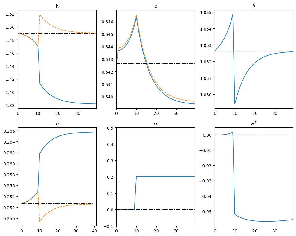
When capital \({k_t}\) decreases in the domestic country after the tax shock, the rental rate \(\eta_t\) increases in that country.
This happens because when capital becomes scarcer, its marginal product rises.