108. Maximum Likelihood Estimation#
GPU
This lecture was built using a machine with access to a GPU — although it will also run without one.
Google Colab has a free tier with GPUs that you can access as follows:
Click on the “play” icon top right
Select Colab
Set the runtime environment to include a GPU
108.1. Overview#
In Linear Regression in Python, we estimated the relationship between dependent and explanatory variables using linear regression.
But what if a linear relationship is not an appropriate assumption for our model?
One widely used alternative is maximum likelihood estimation, which involves specifying a class of distributions, indexed by unknown parameters, and then using the data to pin down these parameter values.
The benefit relative to linear regression is that it allows more flexibility in the probabilistic relationships between variables.
Here we illustrate maximum likelihood by replicating Daniel Treisman’s (2016) paper, Russia’s Billionaires, which connects the number of billionaires in a country to its economic characteristics.
The paper concludes that Russia has a higher number of billionaires than economic factors such as market size and tax rate predict.
We’ll require the following imports:
import numpy as np
import jax.numpy as jnp
import jax
import pandas as pd
from typing import NamedTuple

from jax.scipy.special import factorial, gammaln
from jax.scipy.stats import norm

from statsmodels.api import Poisson
from statsmodels.iolib.summary2 import summary_col

import matplotlib.pyplot as plt
from mpl_toolkits.mplot3d import Axes3D
108.1.1. Prerequisites#
We assume familiarity with basic probability and multivariate calculus.
108.2. Set up and assumptions#
Let’s consider the steps we need to go through in maximum likelihood estimation and how they pertain to this study.
108.2.1. Flow of ideas#
The first step with maximum likelihood estimation is to choose the probability distribution believed to be generating the data.
More precisely, we need to make an assumption as to which parametric class of distributions is generating the data.
e.g., the class of all normal distributions, or the class of all gamma distributions.
Each such class is a family of distributions indexed by a finite number of parameters.
e.g., the class of normal distributions is a family of distributions indexed by its mean \(\mu \in (-\infty, \infty)\) and standard deviation \(\sigma \in (0, \infty)\).
We’ll let the data pick out a particular element of the class by pinning down the parameters.
The parameter estimates so produced will be called maximum likelihood estimates.
108.2.2. Counting billionaires#
Treisman [Treisman, 2016] is interested in estimating the number of billionaires in different countries.
The number of billionaires is integer-valued.
Hence we consider distributions that take values only in the nonnegative integers.
(This is one reason least squares regression is not the best tool for the present problem, since the dependent variable in linear regression is not restricted to integer values.)
One integer distribution is the Poisson distribution, the probability mass function (pmf) of which is
We can plot the Poisson distribution over \(y\) for different values of \(\mu\) as follows
@jax.jit
def poisson_pmf(y, μ):
    return μ**y / factorial(y) * jnp.exp(-μ)
y_values = range(0, 25)

fig, ax = plt.subplots(figsize=(12, 8))

for μ in [1, 5, 10]:
    distribution = []
    for y_i in y_values:
        distribution.append(poisson_pmf(y_i, μ))
    ax.plot(
        y_values,
        distribution,
        label=rf"$\mu$={μ}",
        alpha=0.5,
        marker="o",
        markersize=8,
    )

ax.grid()
ax.set_xlabel(r"$y$", fontsize=14)
ax.set_ylabel(r"$f(y \mid \mu)$", fontsize=14)
ax.axis(xmin=0, ymin=0)
ax.legend(fontsize=14)

plt.show()
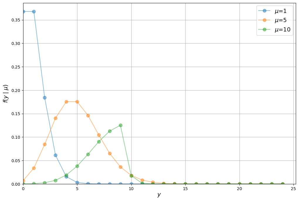
Notice that the Poisson distribution begins to resemble a normal distribution as the mean of \(y\) increases.
Let’s have a look at the distribution of the data we’ll be working with in this lecture.
Treisman’s main source of data is Forbes’ annual rankings of billionaires and their estimated net worth.
The dataset mle/fp.dta can be downloaded from here
or its AER page.
# Load in data and view
df = pd.read_stata(
    "https://github.com/QuantEcon/lecture-python.myst/raw/refs/heads/main/lectures/_static/lecture_specific/mle/fp.dta"
)
df.head()
| country | ccode | year | cyear | numbil | numbil0 | numbilall | netw | netw0 | netwall | ... | gattwto08 | mcapbdol | mcapbdol08 | lnmcap08 | topintaxnew | topint08 | rintr | noyrs | roflaw | nrrents | |
|---|---|---|---|---|---|---|---|---|---|---|---|---|---|---|---|---|---|---|---|---|---|
| 0 | United States | 2.0 | 1990.0 | 21990.0 | NaN | NaN | NaN | NaN | NaN | NaN | ... | 0.0 | 3060.000000 | 11737.599609 | 9.370638 | 39.799999 | 39.799999 | 4.988405 | 20.0 | 1.61 | NaN |
| 1 | United States | 2.0 | 1991.0 | 21991.0 | NaN | NaN | NaN | NaN | NaN | NaN | ... | 0.0 | 4090.000000 | 11737.599609 | 9.370638 | 39.799999 | 39.799999 | 4.988405 | 20.0 | 1.61 | NaN |
| 2 | United States | 2.0 | 1992.0 | 21992.0 | NaN | NaN | NaN | NaN | NaN | NaN | ... | 0.0 | 4490.000000 | 11737.599609 | 9.370638 | 39.799999 | 39.799999 | 4.988405 | 20.0 | 1.61 | NaN |
| 3 | United States | 2.0 | 1993.0 | 21993.0 | NaN | NaN | NaN | NaN | NaN | NaN | ... | 0.0 | 5136.198730 | 11737.599609 | 9.370638 | 39.799999 | 39.799999 | 4.988405 | 20.0 | 1.61 | NaN |
| 4 | United States | 2.0 | 1994.0 | 21994.0 | NaN | NaN | NaN | NaN | NaN | NaN | ... | 0.0 | 5067.016113 | 11737.599609 | 9.370638 | 39.799999 | 39.799999 | 4.988405 | 20.0 | 1.61 | NaN |
5 rows × 36 columns
Using a histogram, we can view the distribution of the number of
billionaires per country, numbil0, in 2008 (the United States is
dropped for plotting purposes)
numbil0_2008 = df[
    (df["year"] == 2008) & (df["country"] != "United States")
].loc[:, "numbil0"]

plt.subplots(figsize=(12, 8))
plt.hist(numbil0_2008, bins=30)
plt.xlim(left=0)
plt.grid()
plt.xlabel("Number of billionaires in 2008")
plt.ylabel("Count")
plt.show()
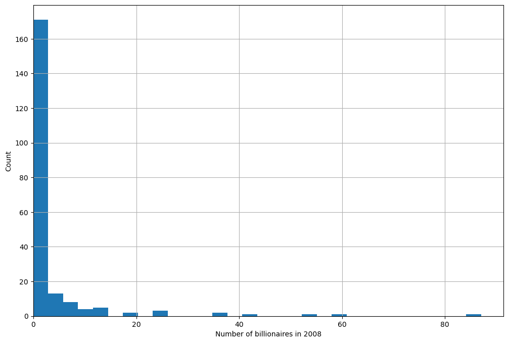
From the histogram, it appears that the Poisson assumption is not unreasonable (albeit with a very low \(\mu\) and some outliers).
108.3. Conditional distributions#
In Treisman’s paper, the dependent variable — the number of billionaires \(y_i\) in country \(i\) — is modeled as a function of GDP per capita, population size, and years membership in GATT and WTO.
Hence, the distribution of \(y_i\) needs to be conditioned on the vector of explanatory variables \(\mathbf{x}_i\).
The standard formulation — the so-called Poisson regression model — is as follows:
To illustrate the idea that the distribution of \(y_i\) depends on \(\mathbf{x}_i\) let’s run a simple simulation.
We use our poisson_pmf function from above and arbitrary values for
\(\boldsymbol{\beta}\) and \(\mathbf{x}_i\)
y_values = range(0, 20)

# Define a parameter vector with estimates
β = jnp.array([0.26, 0.18, 0.25, -0.1, -0.22])

# Create some observations X
datasets = [
    jnp.array([0, 1, 1, 1, 2]),
    jnp.array([2, 3, 2, 4, 0]),
    jnp.array([3, 4, 5, 3, 2]),
    jnp.array([6, 5, 4, 4, 7]),
]


fig, ax = plt.subplots(figsize=(12, 8))

for X in datasets:
    μ = jnp.exp(X @ β)
    distribution = []
    for y_i in y_values:
        distribution.append(poisson_pmf(y_i, μ))
    ax.plot(
        y_values,
        distribution,
        label=rf"$\mu_i$={μ:.1}",
        marker="o",
        markersize=8,
        alpha=0.5,
    )

ax.grid()
ax.legend()
ax.set_xlabel(r"$y \mid x_i$")
ax.set_ylabel(r"$f(y \mid x_i; \beta )$")
ax.axis(xmin=0, ymin=0)
plt.show()
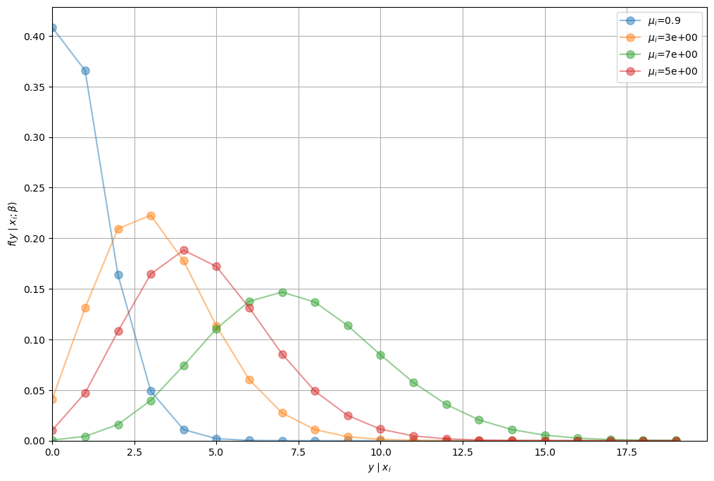
We can see that the distribution of \(y_i\) is conditional on \(\mathbf{x}_i\) (\(\mu_i\) is no longer constant).
108.4. Maximum likelihood estimation#
In our model for number of billionaires, the conditional distribution contains 4 (\(k = 4\)) parameters that we need to estimate.
We will label our entire parameter vector as \(\boldsymbol{\beta}\) where
To estimate the model using MLE, we want to maximize the likelihood that our estimate \(\hat{\boldsymbol{\beta}}\) is the true parameter \(\boldsymbol{\beta}\).
Intuitively, we want to find the \(\hat{\boldsymbol{\beta}}\) that best fits our data.
First, we need to construct the likelihood function \(\mathcal{L}(\boldsymbol{\beta})\), which is similar to a joint probability density function.
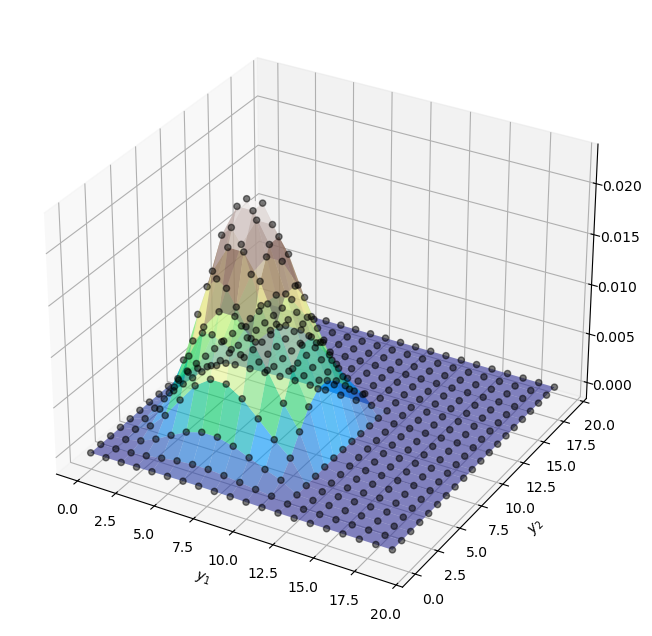
Assume we have some data \(y_i = \{y_1, y_2\}\) and \(y_i \sim f(y_i)\).
If \(y_1\) and \(y_2\) are independent, the joint pmf of these data is \(f(y_1, y_2) = f(y_1) \cdot f(y_2)\).
If \(y_i\) follows a Poisson distribution with \(\lambda = 7\), we can visualize the joint pmf like so
def plot_joint_poisson(μ=7, y_n=20):
    yi_values = jnp.arange(0, y_n, 1)

    # Create coordinate points of X and Y
    X, Y = jnp.meshgrid(yi_values, yi_values)

    # Multiply distributions together
    Z = poisson_pmf(X, μ) * poisson_pmf(Y, μ)

    fig = plt.figure(figsize=(12, 8))
    ax = fig.add_subplot(111, projection="3d")
    ax.plot_surface(X, Y, Z.T, cmap="terrain", alpha=0.6)
    ax.scatter(X, Y, Z.T, color="black", alpha=0.5, linewidths=1)
    ax.set(xlabel=r"$y_1$", ylabel=r"$y_2$")
    ax.set_zlabel(r"$f(y_1, y_2)$", labelpad=10)
    plt.show()


plot_joint_poisson(μ=7, y_n=20)
Similarly, the joint pmf of our data (which is distributed as a conditional Poisson distribution) can be written as
\(y_i\) is conditional on both the values of \(\mathbf{x}_i\) and the parameters \(\boldsymbol{\beta}\).
The likelihood function is the same as the joint pmf, but treats the parameter \(\boldsymbol{\beta}\) as a random variable and takes the observations \((y_i, \mathbf{x}_i)\) as given
Now that we have our likelihood function, we want to find the \(\hat{\boldsymbol{\beta}}\) that yields the maximum likelihood value
In doing so it is generally easier to maximize the log-likelihood (consider differentiating \(f(x) = x \exp(x)\) vs. \(f(x) = \log(x) + x\)).
Given that taking a logarithm is a monotone increasing transformation, a maximizer of the likelihood function will also be a maximizer of the log-likelihood function.
In our case the log-likelihood is
The MLE of the Poisson for \(\hat{\beta}\) can be obtained by solving
However, no analytical solution exists to the above problem – to find the MLE we need to use numerical methods.
108.5. MLE with numerical methods#
Many distributions do not have nice, analytical solutions and therefore require numerical methods to solve for parameter estimates.
One such numerical method is the Newton-Raphson algorithm.
Our goal is to find the maximum likelihood estimate \(\hat{\boldsymbol{\beta}}\).
At \(\hat{\boldsymbol{\beta}}\), the first derivative of the log-likelihood function will be equal to 0.
Let’s illustrate this by supposing
@jax.jit
def logL(β):
    return -((β - 10) ** 2) - 10
To find the value of the gradient of the above function, we can use jax.grad which auto-differentiates the given function.
We further use jax.vmap which vectorizes the given function i.e. the function acting upon scalar inputs can now be used with vector inputs.
dlogL = jax.vmap(jax.grad(logL))
β = jnp.linspace(1, 20)

fig, (ax1, ax2) = plt.subplots(2, sharex=True, figsize=(12, 8))

ax1.plot(β, logL(β), lw=2)
ax2.plot(β, dlogL(β), lw=2)

ax1.set_ylabel(
    r"$log \mathcal{L(\beta)}$", rotation=0, labelpad=35, fontsize=15
)
ax2.set_ylabel(
    r"$\frac{dlog \mathcal{L(\beta)}}{d \beta}$ ",
    rotation=0,
    labelpad=35,
    fontsize=19,
)
ax2.set_xlabel(r"$\beta$", fontsize=15)
ax1.grid(), ax2.grid()
plt.axhline(c="black")
plt.show()
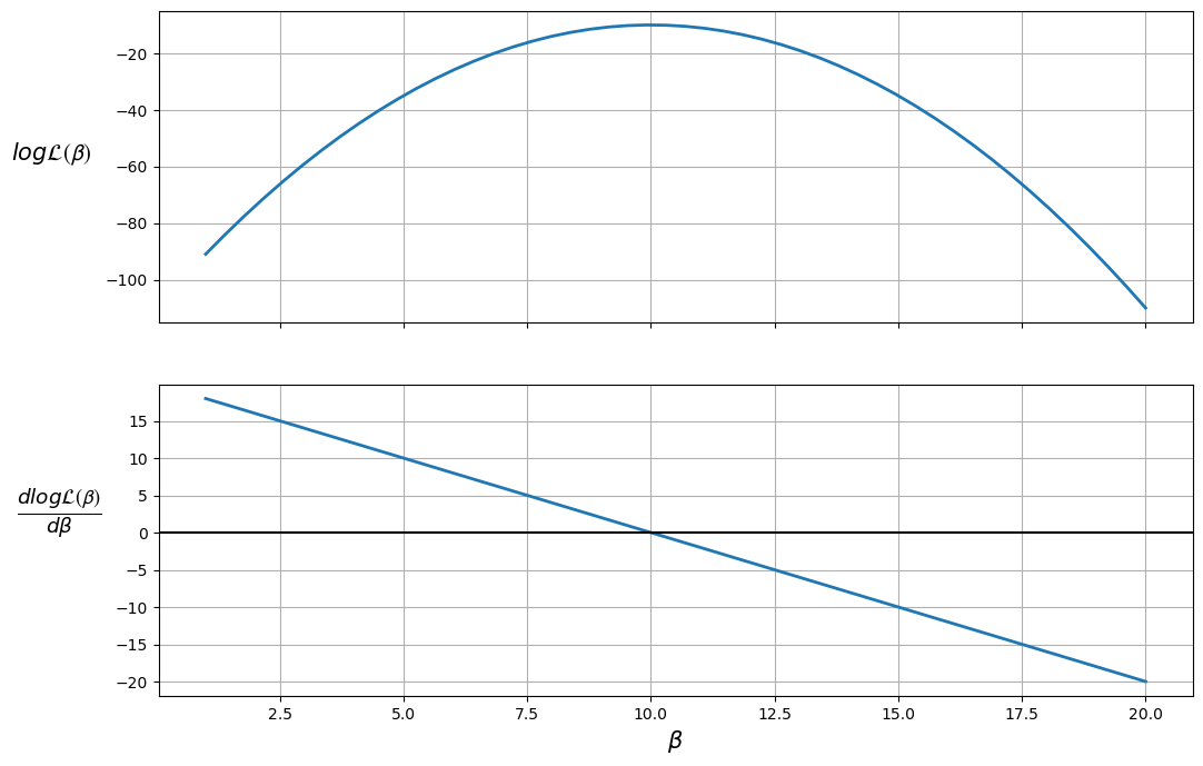
The plot shows that the maximum likelihood value (the top plot) occurs when \(\frac{d \log \mathcal{L(\boldsymbol{\beta})}}{d \boldsymbol{\beta}} = 0\) (the bottom plot).
Therefore, the likelihood is maximized when \(\beta = 10\).
We can also ensure that this value is a maximum (as opposed to a minimum) by checking that the second derivative (slope of the bottom plot) is negative.
The Newton-Raphson algorithm finds a point where the first derivative is 0.
To use the algorithm, we take an initial guess at the maximum value, \(\beta_0\) (the OLS parameter estimates might be a reasonable guess), then
Use the updating rule to iterate the algorithm
\[ \boldsymbol{\beta}_{(k+1)} = \boldsymbol{\beta}_{(k)} - H^{-1}(\boldsymbol{\beta}_{(k)})G(\boldsymbol{\beta}_{(k)}) \]where:
\[\begin{split} \begin{aligned} G(\boldsymbol{\beta}_{(k)}) = \frac{d \log \mathcal{L(\boldsymbol{\beta}_{(k)})}}{d \boldsymbol{\beta}_{(k)}} \\ H(\boldsymbol{\beta}_{(k)}) = \frac{d^2 \log \mathcal{L(\boldsymbol{\beta}_{(k)})}}{d \boldsymbol{\beta}_{(k)}d \boldsymbol{\beta}'_{(k)}} \end{aligned} \end{split}\]Check whether \(\boldsymbol{\beta}_{(k+1)} - \boldsymbol{\beta}_{(k)} < tol\)
If true, then stop iterating and set \(\hat{\boldsymbol{\beta}} = \boldsymbol{\beta}_{(k+1)}\)
If false, then update \(\boldsymbol{\beta}_{(k+1)}\)
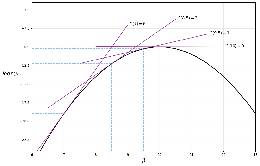
As can be seen from the updating equation, \(\boldsymbol{\beta}_{(k+1)} = \boldsymbol{\beta}_{(k)}\) only when \(G(\boldsymbol{\beta}_{(k)}) = 0\) i.e. where the first derivative is equal to 0.
(In practice, we stop iterating when the difference is below a small tolerance threshold.)
Let’s have a go at implementing the Newton-Raphson algorithm.
First, we’ll create a class called PoissonRegression so we can
easily recompute the values of the log likelihood, gradient and Hessian
for every iteration
class PoissonRegression(NamedTuple):
    X: jnp.ndarray
    y: jnp.ndarray
Now we can define the log likelihood function in Python
@jax.jit
def logL(β, model):
    y = model.y
    μ = jnp.exp(model.X @ β)
    return jnp.sum(model.y * jnp.log(μ) - μ - jnp.log(factorial(y)))
To find the gradient of the poisson_logL, we again use jax.grad.
According to the documentation,
jax.jacfwduses forward-mode automatic differentiation, which is more efficient for “tall” Jacobian matrices, whilejax.jacrevuses reverse-mode, which is more efficient for “wide” Jacobian matrices.
(The documentation also states that when matrices that are near-square, jax.jacfwd probably has an edge over jax.jacrev.)
Therefore, to find the Hessian, we can directly use jax.jacfwd.
G_logL = jax.grad(logL)
H_logL = jax.jacfwd(G_logL)
Our function newton_raphson will take a PoissonRegression object
that has an initial guess of the parameter vector \(\boldsymbol{\beta}_0\).
The algorithm will update the parameter vector according to the updating rule, and recalculate the gradient and Hessian matrices at the new parameter estimates.
Iteration will end when either:
The difference between the parameter and the updated parameter is below a tolerance level.
The maximum number of iterations has been achieved (meaning convergence is not achieved).
So we can get an idea of what’s going on while the algorithm is running,
an option display=True is added to print out values at each
iteration.
def newton_raphson(model, β, tol=1e-3, max_iter=100, display=True):

    i = 0
    error = 100  # Initial error value

    # Print header of output
    if display:
        header = f'{"Iteration_k":<13}{"Log-likelihood":<16}{"θ":<60}'
        print(header)
        print("-" * len(header))

    # While loop runs while any value in error is greater
    # than the tolerance until max iterations are reached
    while jnp.any(error > tol) and i < max_iter:
        H, G = jnp.squeeze(H_logL(β, model)), G_logL(β, model)
        β_new = β - (jnp.dot(jnp.linalg.inv(H), G))
        error = jnp.abs(β_new - β)
        β = β_new

        if display:
            β_list = [f"{t:.3}" for t in list(β.flatten())]
            update = f"{i:<13}{logL(β, model):<16.8}{β_list}"
            print(update)

        i += 1

    print(f"Number of iterations: {i}")
    print(f"β_hat = {β.flatten()}")

    return β
Let’s try out our algorithm with a small dataset of 5 observations and 3 variables in \(\mathbf{X}\).
X = jnp.array([[1, 2, 5], [1, 1, 3], [1, 4, 2], [1, 5, 2], [1, 3, 1]])

y = jnp.array([1, 0, 1, 1, 0])

# Take a guess at initial βs
init_β = jnp.array([0.1, 0.1, 0.1])

# Create an object with Poisson model values
poi = PoissonRegression(X=X, y=y)

# Use newton_raphson to find the MLE
β_hat = newton_raphson(poi, init_β, display=True)
Iteration_k  Log-likelihood  θ
-----------------------------------------------------------------------------------------
0            -4.3447633      ['-1.49', '0.265', '0.244']
1            -3.5742409      ['-3.38', '0.528', '0.474']
2            -3.3999527      ['-5.06', '0.782', '0.702']
3            -3.3788645      ['-5.92', '0.909', '0.82']
4            -3.3783555      ['-6.07', '0.933', '0.843']
5            -3.3783557      ['-6.08', '0.933', '0.843']
6            -3.3783557      ['-6.08', '0.933', '0.843']
Number of iterations: 7
β_hat = [-6.078486   0.9334028  0.8432968]
As this was a simple model with few observations, the algorithm achieved convergence in only 7 iterations.
You can see that with each iteration, the log-likelihood value increased.
Remember, our objective was to maximize the log-likelihood function, which the algorithm has worked to achieve.
Also, note that the increase in \(\log \mathcal{L}(\boldsymbol{\beta}_{(k)})\) becomes smaller with each iteration.
This is because the gradient is approaching 0 as we reach the maximum, and therefore the numerator in our updating equation is becoming smaller.
The gradient vector should be close to 0 at \(\hat{\boldsymbol{\beta}}\)
G_logL(β_hat, poi)
Array([ 7.4505806e-09, -2.9802322e-07, 3.7252903e-08], dtype=float32)
The iterative process can be visualized in the following diagram, where the maximum is found at \(\beta = 10\)
@jax.jit
def logL(x):
    return -((x - 10) ** 2) - 10


@jax.jit
def find_tangent(β, a=0.01):
    y1 = logL(β)
    y2 = logL(β + a)
    x = jnp.array([[β, 1], [β + a, 1]])
    m, c = jnp.linalg.lstsq(x, jnp.array([y1, y2]), rcond=None)[0]
    return m, c
β = jnp.linspace(2, 18)
fig, ax = plt.subplots(figsize=(12, 8))
ax.plot(β, logL(β), lw=2, c="black")

for β in [7, 8.5, 9.5, 10]:
    β_line = jnp.linspace(β - 2, β + 2)
    m, c = find_tangent(β)
    y = m * β_line + c
    ax.plot(β_line, y, "-", c="purple", alpha=0.8)
    ax.text(β + 2.05, y[-1], rf"$G({β}) = {abs(m):.0f}$", fontsize=12)
    ax.vlines(β, -24, logL(β), linestyles="--", alpha=0.5)
    ax.hlines(logL(β), 6, β, linestyles="--", alpha=0.5)

ax.set(ylim=(-24, -4), xlim=(6, 13))
ax.set_xlabel(r"$\beta$", fontsize=15)
ax.set_ylabel(
    r"$log \mathcal{L(\beta)}$", rotation=0, labelpad=25, fontsize=15
)
ax.grid(alpha=0.3)
plt.show()
Note that our implementation of the Newton-Raphson algorithm is rather basic — for more robust implementations see, for example, scipy.optimize.
108.6. Maximum likelihood estimation with statsmodels#
Now that we know what’s going on under the hood, we can apply MLE to an interesting application.
We’ll use the Poisson regression model in statsmodels to obtain
a richer output with standard errors, test values, and more.
statsmodels uses the same algorithm as above to find the maximum
likelihood estimates.
Before we begin, let’s re-estimate our simple model with statsmodels
to confirm we obtain the same coefficients and log-likelihood value.
Now, as statsmodels accepts only NumPy arrays, we can use np.array method
to convert them to NumPy arrays.
X = jnp.array([[1, 2, 5], [1, 1, 3], [1, 4, 2], [1, 5, 2], [1, 3, 1]])

y = jnp.array([1, 0, 1, 1, 0])

y_numpy = np.array(y)
X_numpy = np.array(X)
stats_poisson = Poisson(y_numpy, X_numpy).fit()
print(stats_poisson.summary())
Optimization terminated successfully.
         Current function value: 0.675671
         Iterations 7
                          Poisson Regression Results
==============================================================================
Dep. Variable:                      y   No. Observations:                    5
Model:                        Poisson   Df Residuals:                        2
Method:                           MLE   Df Model:                            2
Date:                Mon, 11 May 2026   Pseudo R-squ.:                  0.2546
Time:                        05:31:40   Log-Likelihood:                -3.3784
converged:                       True   LL-Null:                       -4.5325
Covariance Type:            nonrobust   LLR p-value:                    0.3153
==============================================================================
                 coef    std err          z      P>|z|      [0.025      0.975]
------------------------------------------------------------------------------
const         -6.0785      5.279     -1.151      0.250     -16.425       4.268
x1             0.9334      0.829      1.126      0.260      -0.691       2.558
x2             0.8433      0.798      1.057      0.291      -0.720       2.407
==============================================================================
Now let’s replicate results from Daniel Treisman’s paper, Russia’s Billionaires, mentioned earlier in the lecture.
Treisman starts by estimating equation (108.1), where:
\(y_i\) is \({number\ of\ billionaires}_i\)
\(x_{i1}\) is \(\log{GDP\ per\ capita}_i\)
\(x_{i2}\) is \(\log{population}_i\)
\(x_{i3}\) is \({years\ in\ GATT}_i\) – years membership in GATT and WTO (to proxy access to international markets)
The paper only considers the year 2008 for estimation.
We will set up our variables for estimation like so (you should have the
data assigned to df from earlier in the lecture)
# Keep only year 2008
df = df[df["year"] == 2008]

# Add a constant
df["const"] = 1

# Variable sets
reg1 = ["const", "lngdppc", "lnpop", "gattwto08"]
reg2 = [
    "const",
    "lngdppc",
    "lnpop",
    "gattwto08",
    "lnmcap08",
    "rintr",
    "topint08",
]
reg3 = [
    "const",
    "lngdppc",
    "lnpop",
    "gattwto08",
    "lnmcap08",
    "rintr",
    "topint08",
    "nrrents",
    "roflaw",
]
Then we can use the Poisson function from statsmodels to fit the
model.
We’ll use robust standard errors as in the author’s paper
# Specify model
poisson_reg = Poisson(df[["numbil0"]], df[reg1], missing="drop").fit(
    cov_type="HC0"
)
print(poisson_reg.summary())
Optimization terminated successfully.
         Current function value: 2.226090
         Iterations 9
                          Poisson Regression Results
==============================================================================
Dep. Variable:                numbil0   No. Observations:                  197
Model:                        Poisson   Df Residuals:                      193
Method:                           MLE   Df Model:                            3
Date:                Mon, 11 May 2026   Pseudo R-squ.:                  0.8574
Time:                        05:31:40   Log-Likelihood:                -438.54
converged:                       True   LL-Null:                       -3074.7
Covariance Type:                  HC0   LLR p-value:                     0.000
==============================================================================
                 coef    std err          z      P>|z|      [0.025      0.975]
------------------------------------------------------------------------------
const        -29.0495      2.578    -11.268      0.000     -34.103     -23.997
lngdppc        1.0839      0.138      7.834      0.000       0.813       1.355
lnpop          1.1714      0.097     12.024      0.000       0.980       1.362
gattwto08      0.0060      0.007      0.868      0.386      -0.008       0.019
==============================================================================
Success! The algorithm was able to achieve convergence in 9 iterations.
Our output indicates that GDP per capita, population, and years of membership in the General Agreement on Tariffs and Trade (GATT) are positively related to the number of billionaires a country has, as expected.
Let’s also estimate the author’s more full-featured models and display them in a single table
regs = [reg1, reg2, reg3]
reg_names = ["Model 1", "Model 2", "Model 3"]
info_dict = {
    "Pseudo R-squared": lambda x: f"{x.prsquared:.2f}",
    "No. observations": lambda x: f"{int(x.nobs):d}",
}
regressor_order = [
    "const",
    "lngdppc",
    "lnpop",
    "gattwto08",
    "lnmcap08",
    "rintr",
    "topint08",
    "nrrents",
    "roflaw",
]
results = []

for reg in regs:
    result = Poisson(df[["numbil0"]], df[reg], missing="drop").fit(
        cov_type="HC0", maxiter=100, disp=0
    )
    results.append(result)

results_table = summary_col(
    results=results,
    float_format="%0.3f",
    stars=True,
    model_names=reg_names,
    info_dict=info_dict,
    regressor_order=regressor_order,
)
results_table.add_title(
    "Table 1 - Explaining the Number of Billionaires \
                        in 2008"
)
print(results_table)
Table 1 - Explaining the Number of Billionaires                         in 2008
=================================================
                  Model 1    Model 2    Model 3
-------------------------------------------------
const            -29.050*** -19.444*** -20.858***
                 (2.578)    (4.820)    (4.255)
lngdppc          1.084***   0.717***   0.737***
                 (0.138)    (0.244)    (0.233)
lnpop            1.171***   0.806***   0.929***
                 (0.097)    (0.213)    (0.195)
gattwto08        0.006      0.007      0.004
                 (0.007)    (0.006)    (0.006)
lnmcap08                    0.399**    0.286*
                            (0.172)    (0.167)
rintr                       -0.010     -0.009
                            (0.010)    (0.010)
topint08                    -0.051***  -0.058***
                            (0.011)    (0.012)
nrrents                                -0.005
                                       (0.010)
roflaw                                 0.203
                                       (0.372)
No. observations 197        131        131
Pseudo R-squared 0.86       0.90       0.90
=================================================
Standard errors in parentheses.
* p<.1, ** p<.05, ***p<.01
The output suggests that the frequency of billionaires is positively correlated with GDP per capita, population size, stock market capitalization, and negatively correlated with top marginal income tax rate.
To analyze our results by country, we can plot the difference between the predicted and actual values, then sort from highest to lowest and plot the first 15
data = [
    "const",
    "lngdppc",
    "lnpop",
    "gattwto08",
    "lnmcap08",
    "rintr",
    "topint08",
    "nrrents",
    "roflaw",
    "numbil0",
    "country",
]
results_df = df[data].dropna()

# Use last model (model 3)
results_df["prediction"] = results[-1].predict()

# Calculate difference
results_df["difference"] = results_df["numbil0"] - results_df["prediction"]

# Sort in descending order
results_df.sort_values("difference", ascending=False, inplace=True)

# Plot the first 15 data points
results_df[:15].plot(
    "country", "difference", kind="bar", figsize=(12, 8), legend=False
)
plt.ylabel("Number of billionaires above predicted level")
plt.xlabel("Country")
plt.show()
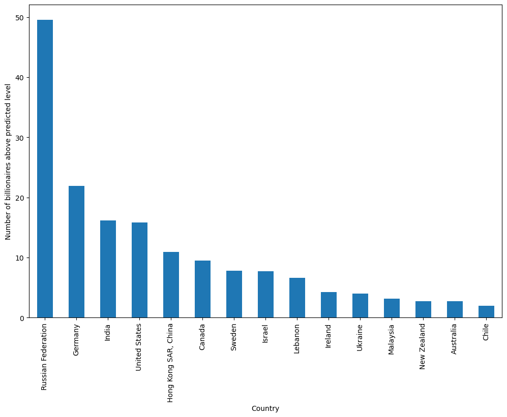
As we can see, Russia has by far the highest number of billionaires in excess of what is predicted by the model (around 50 more than expected).
Treisman uses this empirical result to discuss possible reasons for Russia’s excess of billionaires, including the origination of wealth in Russia, the political climate, and the history of privatization in the years after the USSR.
108.7. Summary#
In this lecture, we used Maximum Likelihood Estimation to estimate the parameters of a Poisson model.
statsmodels contains other built-in likelihood models such as
Probit
and
Logit.
For further flexibility, statsmodels provides a way to specify the
distribution manually using the GenericLikelihoodModel class - an
example notebook can be found
here.
108.8. Exercises#
Exercise 108.1
Suppose we wanted to estimate the probability of an event \(y_i\) occurring, given some observations.
We could use a probit regression model, where the pmf of \(y_i\) is
\(\Phi\) represents the cumulative normal distribution and constrains the predicted \(y_i\) to be between 0 and 1 (as required for a probability).
\(\boldsymbol{\beta}\) is a vector of coefficients.
Following the example in the lecture, write a class to represent the Probit model.
To begin, find the log-likelihood function and derive the gradient and Hessian.
The jax.scipy.stats module norm contains the functions needed to
compute the cdf and pdf of the normal distribution.
Solution
The log-likelihood can be written as
Using the fundamental theorem of calculus, the derivative of a cumulative probability distribution is its marginal distribution
where \(\phi\) is the marginal normal distribution.
The gradient vector of the Probit model is
The Hessian of the Probit model is
Using these results, we can write a class for the Probit model as follows
class ProbitRegression(NamedTuple):
    X: jnp.ndarray
    y: jnp.ndarray
@jax.jit
def logL(β, model):
    y = model.y
    μ = norm.cdf(model.X @ β.T)
    return y @ jnp.log(μ) + (1 - y) @ jnp.log(1 - μ)
G_logL = jax.grad(logL)
H_logL = jax.jacfwd(G_logL)
Exercise 108.2
Use the following dataset and initial values of \(\boldsymbol{\beta}\) to estimate the MLE with the Newton-Raphson algorithm developed earlier in the lecture
Verify your results with statsmodels - you can import the Probit
function with the following import statement
from statsmodels.discrete.discrete_model import Probit
Note that the simple Newton-Raphson algorithm developed in this lecture is very sensitive to initial values, and therefore you may fail to achieve convergence with different starting values.
Solution
Here is one solution
X = jnp.array([[1, 2, 4], [1, 1, 1], [1, 4, 3], [1, 5, 6], [1, 3, 5]])

y = jnp.array([1, 0, 1, 1, 0])

# Take a guess at initial βs
β = jnp.array([0.1, 0.1, 0.1])

# Create a model of Probit regression
prob = ProbitRegression(y=y, X=X)

# Run Newton-Raphson algorithm
newton_raphson(prob, β)
Iteration_k  Log-likelihood  θ
-----------------------------------------------------------------------------------------
0            -2.3796887      ['-1.34', '0.775', '-0.157']
1            -2.3687525      ['-1.53', '0.775', '-0.0981']
2            -2.3687296      ['-1.55', '0.778', '-0.0971']
3            -2.3687291      ['-1.55', '0.778', '-0.0971']
Number of iterations: 4
β_hat = [-1.5462587   0.77778953 -0.09709755]
Array([-1.5462587 , 0.77778953, -0.09709755], dtype=float32)
# Use statsmodels to verify results
y_numpy = np.array(y)
X_numpy = np.array(X)
print(Probit(y_numpy, X_numpy).fit().summary())
Optimization terminated successfully.
         Current function value: 0.473746
         Iterations 6
                          Probit Regression Results
==============================================================================
Dep. Variable:                      y   No. Observations:                    5
Model:                         Probit   Df Residuals:                        2
Method:                           MLE   Df Model:                            2
Date:                Mon, 11 May 2026   Pseudo R-squ.:                  0.2961
Time:                        05:31:42   Log-Likelihood:                -2.3687
converged:                       True   LL-Null:                       -3.3651
Covariance Type:            nonrobust   LLR p-value:                    0.3692
==============================================================================
                 coef    std err          z      P>|z|      [0.025      0.975]
------------------------------------------------------------------------------
const         -1.5463      1.866     -0.829      0.407      -5.204       2.111
x1             0.7778      0.788      0.986      0.324      -0.768       2.323
x2            -0.0971      0.590     -0.165      0.869      -1.254       1.060
==============================================================================