39. Inventory Dynamics#
39.1. Overview#
In this lecture we will study the time path of inventories for firms that follow so-called s-S inventory dynamics.
Such firms
wait until inventory falls below some level \(s\) and then
order sufficient quantities to bring their inventory back up to capacity \(S\).
These kinds of policies are common in practice and also optimal in certain circumstances.
A review of early literature and some macroeconomic implications can be found in [Caplin, 1985].
Here our main aim is to learn more about simulation, time series and Markov dynamics.
While our Markov environment and many of the concepts we consider are related to those found in our lecture on finite Markov chains, the state space is a continuum in the current application.
Let’s start with some imports
import matplotlib.pyplot as plt
import numpy as np
from numba import jit, float64, prange
from numba.experimental import jitclass
39.2. Sample Paths#
Consider a firm with inventory \(X_t\).
The firm waits until \(X_t \leq s\) and then restocks up to \(S\) units.
It faces stochastic demand \(\{ D_t \}\), which we assume is IID.
With notation \(a^+ := \max\{a, 0\}\), inventory dynamics can be written as
In what follows, we will assume that each \(D_t\) is lognormal, so that
where \(\mu\) and \(\sigma\) are parameters and \(\{Z_t\}\) is IID and standard normal.
Here’s a class that stores parameters and generates time paths for inventory.
firm_data = [
   ('s', float64),          # restock trigger level
   ('S', float64),          # capacity
   ('mu', float64),         # shock location parameter
   ('sigma', float64)       # shock scale parameter
]


@jitclass(firm_data)
class Firm:

    def __init__(self, s=10, S=100, mu=1.0, sigma=0.5):

        self.s, self.S, self.mu, self.sigma = s, S, mu, sigma

    def update(self, x):
        "Update the state from t to t+1 given current state x."

        Z = np.random.randn()
        D = np.exp(self.mu + self.sigma * Z)
        if x <= self.s:
            return max(self.S - D, 0)
        else:
            return max(x - D, 0)

    def sim_inventory_path(self, x_init, sim_length):

        X = np.empty(sim_length)
        X[0] = x_init

        for t in range(sim_length-1):
            X[t+1] = self.update(X[t])
        return X
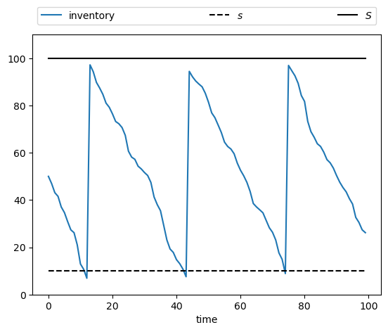
Let’s run a first simulation, of a single path:
firm = Firm()

s, S = firm.s, firm.S
sim_length = 100
x_init = 50

X = firm.sim_inventory_path(x_init, sim_length)

fig, ax = plt.subplots()
bbox = (0., 1.02, 1., .102)
legend_args = {'ncol': 3,
               'bbox_to_anchor': bbox,
               'loc': 3,
               'mode': 'expand'}

ax.plot(X, label="inventory")
ax.plot(np.full(sim_length, s), 'k--', label="$s$")
ax.plot(np.full(sim_length, S), 'k-', label="$S$")
ax.set_ylim(0, S+10)
ax.set_xlabel("time")
ax.legend(**legend_args)

plt.show()
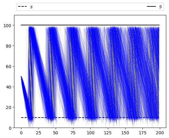
Now let’s simulate multiple paths in order to build a more complete picture of the probabilities of different outcomes:
sim_length=200
fig, ax = plt.subplots()

ax.plot(np.full(sim_length, s), 'k--', label="$s$")
ax.plot(np.full(sim_length, S), 'k-', label="$S$")
ax.set_ylim(0, S+10)
ax.legend(**legend_args)

for i in range(400):
    X = firm.sim_inventory_path(x_init, sim_length)
    ax.plot(X, 'b', alpha=0.2, lw=0.5)

plt.show()
39.3. Marginal Distributions#
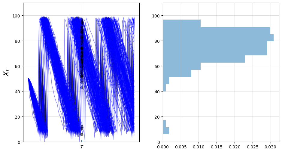
Now let’s look at the marginal distribution \(\psi_T\) of \(X_T\) for some fixed \(T\).
We will do this by generating many draws of \(X_T\) given initial condition \(X_0\).
With these draws of \(X_T\) we can build up a picture of its distribution \(\psi_T\).
Here’s one visualization, with \(T=50\).
T = 50
M = 200  # Number of draws

ymin, ymax = 0, S + 10

fig, axes = plt.subplots(1, 2, figsize=(11, 6))

for ax in axes:
    ax.grid(alpha=0.4)

ax = axes[0]

ax.set_ylim(ymin, ymax)
ax.set_ylabel('$X_t$', fontsize=16)
ax.vlines((T,), -1.5, 1.5)

ax.set_xticks((T,))
ax.set_xticklabels((r'$T$',))

sample = np.empty(M)
for m in range(M):
    X = firm.sim_inventory_path(x_init, 2 * T)
    ax.plot(X, 'b-', lw=1, alpha=0.5)
    ax.plot((T,), (X[T+1],), 'ko', alpha=0.5)
    sample[m] = X[T+1]

axes[1].set_ylim(ymin, ymax)

axes[1].hist(sample,
             bins=16,
             density=True,
             orientation='horizontal',
             histtype='bar',
             alpha=0.5)

plt.show()
We can build up a clearer picture by drawing more samples
T = 50
M = 50_000

fig, ax = plt.subplots()

sample = np.empty(M)
for m in range(M):
    X = firm.sim_inventory_path(x_init, T+1)
    sample[m] = X[T]

ax.hist(sample,
         bins=36,
         density=True,
         histtype='bar',
         alpha=0.75)

plt.show()
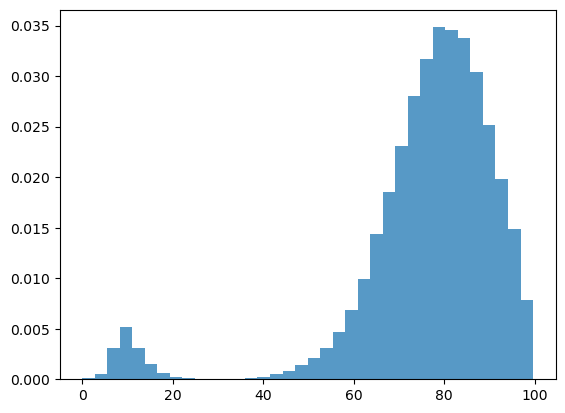
Note that the distribution is bimodal
Most firms have restocked twice but a few have restocked only once (see figure with paths above).
Firms in the second category have lower inventory.
We can also approximate the distribution using a kernel density estimator.
Kernel density estimators can be thought of as smoothed histograms.
They are preferable to histograms when the distribution being estimated is likely to be smooth.
We will use a kernel density estimator from scikit-learn
from sklearn.neighbors import KernelDensity

def plot_kde(sample, ax, label=''):

    xmin, xmax = 0.9 * min(sample), 1.1 * max(sample)
    xgrid = np.linspace(xmin, xmax, 200)
    kde = KernelDensity(kernel='gaussian').fit(sample[:, None])
    log_dens = kde.score_samples(xgrid[:, None])

    ax.plot(xgrid, np.exp(log_dens), label=label)
fig, ax = plt.subplots()
plot_kde(sample, ax)
plt.show()
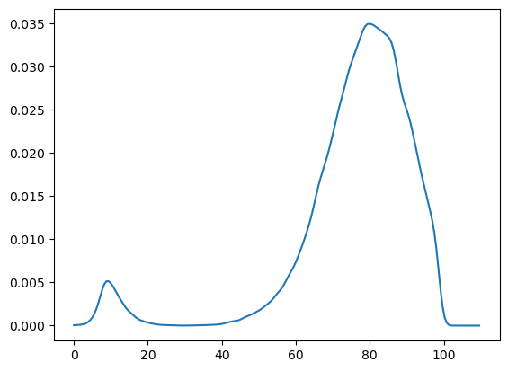
The allocation of probability density is similar to what was shown by the histogram just above.
39.4. Exercises#
Exercise 39.1
This model is asymptotically stationary, with a unique stationary distribution.
(See the discussion of stationarity in our lecture on AR(1) processes for background — the fundamental concepts are the same.)
In particular, the sequence of marginal distributions \(\{\psi_t\}\) is converging to a unique limiting distribution that does not depend on initial conditions.
Although we will not prove this here, we can investigate it using simulation.
Your task is to generate and plot the sequence \(\{\psi_t\}\) at times \(t = 10, 50, 250, 500, 750\) based on the discussion above.
(The kernel density estimator is probably the best way to present each distribution.)
You should see convergence, in the sense that differences between successive distributions are getting smaller.
Try different initial conditions to verify that, in the long run, the distribution is invariant across initial conditions.
Solution
Below is one possible solution:
The computations involve a lot of CPU cycles so we have tried to write the code efficiently.
This meant writing a specialized function rather than using the class above.
s, S, mu, sigma = firm.s, firm.S, firm.mu, firm.sigma

@jit(parallel=True)
def shift_firms_forward(current_inventory_levels, num_periods):

    num_firms = len(current_inventory_levels)
    new_inventory_levels = np.empty(num_firms)

    for f in prange(num_firms):
        x = current_inventory_levels[f]
        for t in range(num_periods):
            Z = np.random.randn()
            D = np.exp(mu + sigma * Z)
            if x <= s:
                x = max(S - D, 0)
            else:
                x = max(x - D, 0)
        new_inventory_levels[f] = x

    return new_inventory_levels
x_init = 50
num_firms = 50_000

sample_dates = 0, 10, 50, 250, 500, 750

first_diffs = np.diff(sample_dates)

fig, ax = plt.subplots()

X = np.full(num_firms, x_init)

current_date = 0
for d in first_diffs:
    X = shift_firms_forward(X, d)
    current_date += d
    plot_kde(X, ax, label=f't = {current_date}')

ax.set_xlabel('inventory')
ax.set_ylabel('probability')
ax.legend()
plt.show()
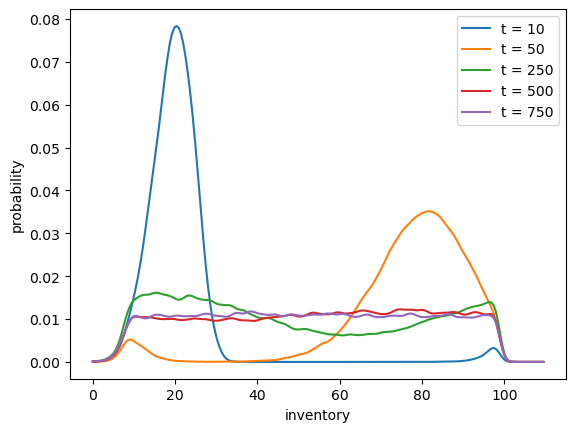
Notice that by \(t=500\) or \(t=750\) the densities are barely changing.
We have reached a reasonable approximation of the stationary density.
You can convince yourself that initial conditions don’t matter by testing a few of them.
For example, try rerunning the code above with all firms starting at \(X_0 = 20\) or \(X_0 = 80\).
Exercise 39.2
Using simulation, calculate the probability that firms that start with \(X_0 = 70\) need to order twice or more in the first 50 periods.
You will need a large sample size to get an accurate reading.
Solution
Here is one solution.
Again, the computations are relatively intensive so we have written a a specialized function rather than using the class above.
We will also use parallelization across firms.
@jit(parallel=True)
def compute_freq(sim_length=50, x_init=70, num_firms=1_000_000):

    firm_counter = 0  # Records number of firms that restock 2x or more
    for m in prange(num_firms):
        x = x_init
        restock_counter = 0  # Will record number of restocks for firm m

        for t in range(sim_length):
            Z = np.random.randn()
            D = np.exp(mu + sigma * Z)
            if x <= s:
                x = max(S - D, 0)
                restock_counter += 1
            else:
                x = max(x - D, 0)

        if restock_counter > 1:
            firm_counter += 1

    return firm_counter / num_firms
Note the time the routine takes to run, as well as the output.
%%time

freq = compute_freq()
print(f"Frequency of at least two stock outs = {freq}")
Frequency of at least two stock outs = 0.447451
CPU times: user 2.95 s, sys: 6.91 ms, total: 2.95 s
Wall time: 714 ms
Try switching the parallel flag to False in the @jit decorator
above.
Depending on your system, the difference can be substantial.
(On our desktop machine, the speed up is by a factor of 5.)