29. Wealth Distribution Dynamics #

Contents

Wealth Distribution Dynamics

29.1. Overview #

This notebook gives an introduction to wealth distribution dynamics, with a focus on

modeling and computing the wealth distribution via simulation,
measures of inequality such as the Lorenz curve and Gini coefficient, and
how inequality is affected by the properties of wage income and returns on assets.

One interesting property of the wealth distribution we discuss is Pareto tails.

The wealth distribution in many countries exhibits a Pareto tail

See this lecture for a definition.
For a review of the empirical evidence, see, for example, [Benhabib and Bisin, 2018].

This is consistent with high concentration of wealth amongst the richest households.

It also gives us a way to quantify such concentration, in terms of the tail index.

One question of interest is whether or not we can replicate Pareto tails from a relatively simple model.

29.1.1. A Note on Assumptions#

The evolution of wealth for any given household depends on their savings behavior.

Modeling such behavior will form an important part of this lecture series.

However, in this particular lecture, we will be content with rather ad hoc (but plausible) savings rules.

We do this to more easily explore the implications of different specifications of income dynamics and investment returns.

At the same time, all of the techniques discussed here can be plugged into models that use optimization to obtain savings rules.

We will use the following imports.

import matplotlib.pyplot as plt
plt.rcParams["figure.figsize"] = (11, 5)  #set default figure size
import numpy as np
import quantecon as qe
from numba import njit, float64, prange
from numba.experimental import jitclass

29.2. Lorenz Curves and the Gini Coefficient #

Before we investigate wealth dynamics, we briefly review some measures of inequality.

29.2.1. Lorenz Curves#

One popular graphical measure of inequality is the Lorenz curve.

The package QuantEcon.py, already imported above, contains a function to compute Lorenz curves.

To illustrate, suppose that

n = 10_000                      # size of sample
w = np.exp(np.random.randn(n))  # lognormal draws

is data representing the wealth of 10,000 households.

We can compute and plot the Lorenz curve as follows:

f_vals, l_vals = qe.lorenz_curve(w)

fig, ax = plt.subplots()
ax.plot(f_vals, l_vals, label='Lorenz curve, lognormal sample')
ax.plot(f_vals, f_vals, label='Lorenz curve, equality')
ax.legend()
plt.show()

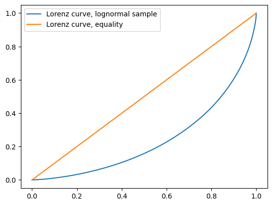
_images/8e2ae98f99449ff9075778c830009b0fc28a19f5cfcad03d2b2e63ad10f99e8f.png

This curve can be understood as follows: if point \((x,y)\) lies on the curve, it means that, collectively, the bottom \((100x)\%\) of the population holds \((100y)\%\) of the wealth.

The “equality” line is the 45 degree line (which might not be exactly 45 degrees in the figure, depending on the aspect ratio).

A sample that produces this line exhibits perfect equality.

The other line in the figure is the Lorenz curve for the lognormal sample, which deviates significantly from perfect equality.

For example, the bottom 80% of the population holds around 40% of total wealth.

Here is another example, which shows how the Lorenz curve shifts as the underlying distribution changes.

We generate 10,000 observations using the Pareto distribution with a range of parameters, and then compute the Lorenz curve corresponding to each set of observations.

a_vals = (1, 2, 5)              # Pareto tail index
n = 10_000                      # size of each sample
fig, ax = plt.subplots()
for a in a_vals:
    u = np.random.uniform(size=n)
    y = u**(-1/a)               # distributed as Pareto with tail index a
    f_vals, l_vals = qe.lorenz_curve(y)
    ax.plot(f_vals, l_vals, label=f'$a = {a}$')
ax.plot(f_vals, f_vals, label='equality')
ax.legend()
plt.show()

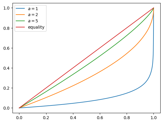
_images/903fc952d605184d47f2d5a9e8e020ff1837fe3ce5408dd1562644792b3eaed7.png

You can see that, as the tail parameter of the Pareto distribution increases, inequality decreases.

This is to be expected, because a higher tail index implies less weight in the tail of the Pareto distribution.

29.2.2. The Gini Coefficient#

The definition and interpretation of the Gini coefficient can be found on the corresponding Wikipedia page.

A value of 0 indicates perfect equality (corresponding the case where the Lorenz curve matches the 45 degree line) and a value of 1 indicates complete inequality (all wealth held by the richest household).

The QuantEcon.py library contains a function to calculate the Gini coefficient.

We can test it on the Weibull distribution with parameter \(a\), where the Gini coefficient is known to be

\[ G = 1 - 2^{-1/a} \]

Let’s see if the Gini coefficient computed from a simulated sample matches this at each fixed value of \(a\).

a_vals = range(1, 20)
ginis = []
ginis_theoretical = []
n = 100

fig, ax = plt.subplots()
for a in a_vals:
    y = np.random.weibull(a, size=n)
    ginis.append(qe.gini_coefficient(y))
    ginis_theoretical.append(1 - 2**(-1/a))
ax.plot(a_vals, ginis, label='estimated gini coefficient')
ax.plot(a_vals, ginis_theoretical, label='theoretical gini coefficient')
ax.legend()
ax.set_xlabel("Weibull parameter $a$")
ax.set_ylabel("Gini coefficient")
plt.show()

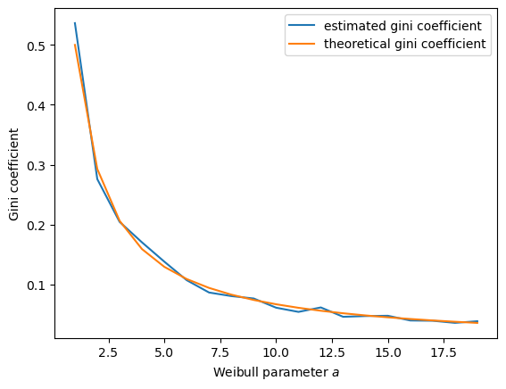
_images/337e1549aca9edd0b1310b985a359ae411e9b8e90610077294b81f415b2b8172.png

The simulation shows that the fit is good.

29.3. A Model of Wealth Dynamics #

Having discussed inequality measures, let us now turn to wealth dynamics.

The model we will study is

(29.1)#\[w_{t+1} = (1 + r_{t+1}) s(w_t) + y_{t+1}\]

where

\(w_t\) is wealth at time \(t\) for a given household,
\(r_t\) is the rate of return of financial assets,
\(y_t\) is current non-financial (e.g., labor) income and
\(s(w_t)\) is current wealth net of consumption

Letting \(\{z_t\}\) be a correlated state process of the form

\[ z_{t+1} = a z_t + b + \sigma_z \epsilon_{t+1} \]

we’ll assume that

\[ R_t := 1 + r_t = c_r \exp(z_t) + \exp(\mu_r + \sigma_r \xi_t) \]

and

\[ y_t = c_y \exp(z_t) + \exp(\mu_y + \sigma_y \zeta_t) \]

Here \(\{ (\epsilon_t, \xi_t, \zeta_t) \}\) is IID and standard normal in \(\mathbb R^3\).

The value of \(c_r\) should be close to zero, since rates of return on assets do not exhibit large trends.

When we simulate a population of households, we will assume all shocks are idiosyncratic (i.e., specific to individual households and independent across them).

Regarding the savings function \(s\), our default model will be

(29.2)#\[s(w) = s_0 w \cdot \mathbb 1\{w \geq \hat w\}\]

where \(s_0\) is a positive constant.

Thus, for \(w < \hat w\), the household saves nothing. For \(w \geq \bar w\), the household saves a fraction \(s_0\) of their wealth.

We are using something akin to a fixed savings rate model, while acknowledging that low wealth households tend to save very little.

29.4. Implementation #

Here’s some type information to help Numba.

wealth_dynamics_data = [
    ('w_hat',  float64),    # savings parameter
    ('s_0',    float64),    # savings parameter
    ('c_y',    float64),    # labor income parameter
    ('μ_y',    float64),    # labor income paraemter
    ('σ_y',    float64),    # labor income parameter
    ('c_r',    float64),    # rate of return parameter
    ('μ_r',    float64),    # rate of return parameter
    ('σ_r',    float64),    # rate of return parameter
    ('a',      float64),    # aggregate shock parameter
    ('b',      float64),    # aggregate shock parameter
    ('σ_z',    float64),    # aggregate shock parameter
    ('z_mean', float64),    # mean of z process
    ('z_var', float64),     # variance of z process
    ('y_mean', float64),    # mean of y process
    ('R_mean', float64)     # mean of R process
]

Here’s a class that stores instance data and implements methods that update the aggregate state and household wealth.

@jitclass(wealth_dynamics_data)
class WealthDynamics:

    def __init__(self,
                 w_hat=1.0,
                 s_0=0.75,
                 c_y=1.0,
                 μ_y=1.0,
                 σ_y=0.2,
                 c_r=0.05,
                 μ_r=0.1,
                 σ_r=0.5,
                 a=0.5,
                 b=0.0,
                 σ_z=0.1):

        self.w_hat, self.s_0 = w_hat, s_0
        self.c_y, self.μ_y, self.σ_y = c_y, μ_y, σ_y
        self.c_r, self.μ_r, self.σ_r = c_r, μ_r, σ_r
        self.a, self.b, self.σ_z = a, b, σ_z

        # Record stationary moments
        self.z_mean = b / (1 - a)
        self.z_var = σ_z**2 / (1 - a**2)
        exp_z_mean = np.exp(self.z_mean + self.z_var / 2)
        self.R_mean = c_r * exp_z_mean + np.exp(μ_r + σ_r**2 / 2)
        self.y_mean = c_y * exp_z_mean + np.exp(μ_y + σ_y**2 / 2)

        # Test a stability condition that ensures wealth does not diverge
        # to infinity.
        α = self.R_mean * self.s_0
        if α >= 1:
            raise ValueError("Stability condition failed.")

    def parameters(self):
        """
        Collect and return parameters.
        """
        parameters = (self.w_hat, self.s_0,
                      self.c_y, self.μ_y, self.σ_y,
                      self.c_r, self.μ_r, self.σ_r,
                      self.a, self.b, self.σ_z)
        return parameters

    def update_states(self, w, z):
        """
        Update one period, given current wealth w and persistent
        state z.
        """

        # Simplify names
        params = self.parameters()
        w_hat, s_0, c_y, μ_y, σ_y, c_r, μ_r, σ_r, a, b, σ_z = params
        zp = a * z + b + σ_z * np.random.randn()

        # Update wealth
        y = c_y * np.exp(zp) + np.exp(μ_y + σ_y * np.random.randn())
        wp = y
        if w >= w_hat:
            R = c_r * np.exp(zp) + np.exp(μ_r + σ_r * np.random.randn())
            wp += R * s_0 * w
        return wp, zp

Here’s function to simulate the time series of wealth for in individual households.

@njit
def wealth_time_series(wdy, w_0, n):
    """
    Generate a single time series of length n for wealth given
    initial value w_0.

    The initial persistent state z_0 for each household is drawn from
    the stationary distribution of the AR(1) process.

        * wdy: an instance of WealthDynamics
        * w_0: scalar
        * n: int


    """
    z = wdy.z_mean + np.sqrt(wdy.z_var) * np.random.randn()
    w = np.empty(n)
    w[0] = w_0
    for t in range(n-1):
        w[t+1], z = wdy.update_states(w[t], z)
    return w

Now here’s function to simulate a cross section of households forward in time.

Note the use of parallelization to speed up computation.

@njit(parallel=True)
def update_cross_section(wdy, w_distribution, shift_length=500):
    """
    Shifts a cross-section of household forward in time

    * wdy: an instance of WealthDynamics
    * w_distribution: array_like, represents current cross-section

    Takes a current distribution of wealth values as w_distribution
    and updates each w_t in w_distribution to w_{t+j}, where
    j = shift_length.

    Returns the new distribution.

    """
    new_distribution = np.empty_like(w_distribution)

    # Update each household
    for i in prange(len(new_distribution)):
        z = wdy.z_mean + np.sqrt(wdy.z_var) * np.random.randn()
        w = w_distribution[i]
        for t in range(shift_length-1):
            w, z = wdy.update_states(w, z)
        new_distribution[i] = w
    return new_distribution

Parallelization is very effective in the function above because the time path of each household can be calculated independently once the path for the aggregate state is known.

29.5. Applications #

Let’s try simulating the model at different parameter values and investigate the implications for the wealth distribution.

29.5.1. Time Series#

Let’s look at the wealth dynamics of an individual household.

wdy = WealthDynamics()
ts_length = 200
w = wealth_time_series(wdy, wdy.y_mean, ts_length)

fig, ax = plt.subplots()
ax.plot(w)
plt.show()

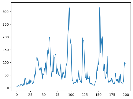
_images/99279e5d80b12cdab632b8f9d94ba5cc6f26d1d8c468c2218b0cf84e6c751e95.png

Notice the large spikes in wealth over time.

Such spikes are similar to what we observed in time series when we studied Kesten processes.

29.5.2. Inequality Measures#

Let’s look at how inequality varies with returns on financial assets.

The next function generates a cross section and then computes the Lorenz curve and Gini coefficient.

def generate_lorenz_and_gini(wdy, num_households=100_000, T=500):
    """
    Generate the Lorenz curve data and gini coefficient corresponding to a
    WealthDynamics mode by simulating num_households forward to time T.
    """
    ψ_0 = np.full(num_households, wdy.y_mean)
    z_0 = wdy.z_mean

    ψ_star = update_cross_section(wdy, ψ_0, shift_length=T)
    return qe.gini_coefficient(ψ_star), qe.lorenz_curve(ψ_star)

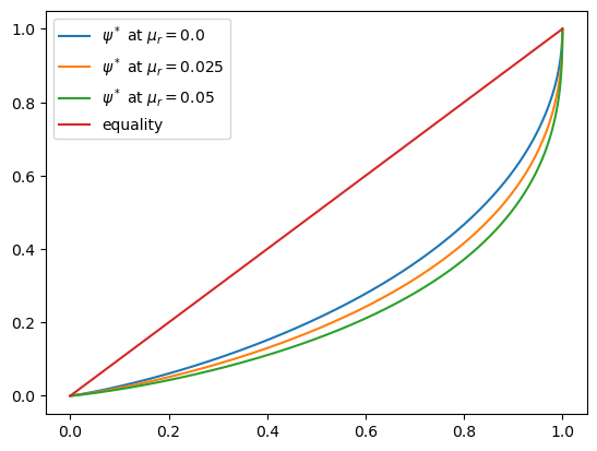
Now we investigate how the Lorenz curves associated with the wealth distribution change as return to savings varies.

The code below plots Lorenz curves for three different values of \(\mu_r\).

If you are running this yourself, note that it will take one or two minutes to execute.

This is unavoidable because we are executing a CPU intensive task.

In fact the code, which is JIT compiled and parallelized, runs extremely fast relative to the number of computations.

%%time

fig, ax = plt.subplots()
μ_r_vals = (0.0, 0.025, 0.05)
gini_vals = []

for μ_r in μ_r_vals:
    wdy = WealthDynamics(μ_r=μ_r)
    gv, (f_vals, l_vals) = generate_lorenz_and_gini(wdy)
    ax.plot(f_vals, l_vals, label=f'$\psi^*$ at $\mu_r = {μ_r:0.2}$')
    gini_vals.append(gv)

ax.plot(f_vals, f_vals, label='equality')
ax.legend(loc="upper left")
plt.show()

_images/1a678e512c52f03bba06c3232765b619b1f95a363029d7bfc2af6b7d763489a6.png

CPU times: user 1min 28s, sys: 31.4 ms, total: 1min 28s
Wall time: 12.3 s

The Lorenz curve shifts downwards as returns on financial income rise, indicating a rise in inequality.

We will look at this again via the Gini coefficient immediately below, but first consider the following image of our system resources when the code above is executing:

Since the code is both efficiently JIT compiled and fully parallelized, it’s close to impossible to make this sequence of tasks run faster without changing hardware.

Now let’s check the Gini coefficient.

fig, ax = plt.subplots()
ax.plot(μ_r_vals, gini_vals, label='gini coefficient')
ax.set_xlabel("$\mu_r$")
ax.legend()
plt.show()

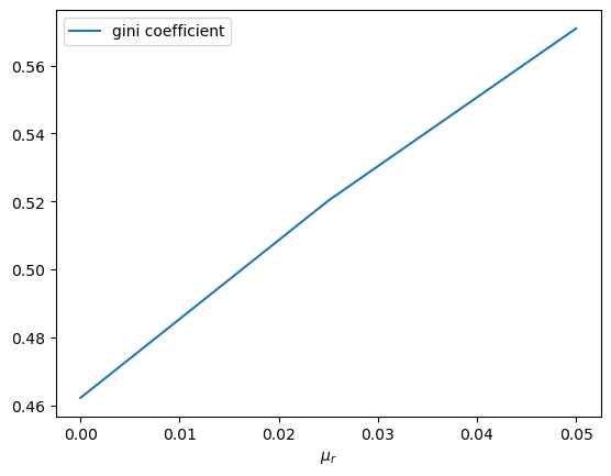
_images/40c33db07f573eda6872e2e9931a1f6c035c0626fb17e3ded1eba5c5ebac725c.png

Once again, we see that inequality increases as returns on financial income rise.

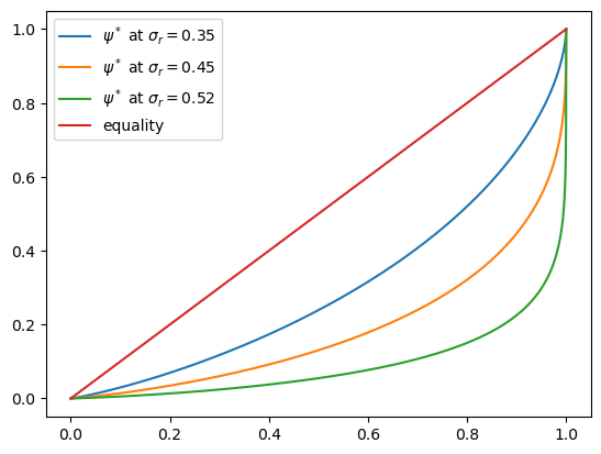
Let’s finish this section by investigating what happens when we change the volatility term \(\sigma_r\) in financial returns.

%%time

fig, ax = plt.subplots()
σ_r_vals = (0.35, 0.45, 0.52)
gini_vals = []

for σ_r in σ_r_vals:
    wdy = WealthDynamics(σ_r=σ_r)
    gv, (f_vals, l_vals) = generate_lorenz_and_gini(wdy)
    ax.plot(f_vals, l_vals, label=f'$\psi^*$ at $\sigma_r = {σ_r:0.2}$')
    gini_vals.append(gv)

ax.plot(f_vals, f_vals, label='equality')
ax.legend(loc="upper left")
plt.show()

_images/bdeaf162249e98073abc1768229c46b4d6e7c3427aaecb615196801001310f04.png

CPU times: user 1min 28s, sys: 55.8 ms, total: 1min 28s
Wall time: 11.4 s

We see that greater volatility has the effect of increasing inequality in this model.

29.6. Exercises #

Exercise 29.1

For a wealth or income distribution with Pareto tail, a higher tail index suggests lower inequality.

Indeed, it is possible to prove that the Gini coefficient of the Pareto distribution with tail index \(a\) is \(1/(2a - 1)\).

To the extent that you can, confirm this by simulation.

In particular, generate a plot of the Gini coefficient against the tail index using both the theoretical value just given and the value computed from a sample via qe.gini_coefficient.

For the values of the tail index, use a_vals = np.linspace(1, 10, 25).

Use sample of size 1,000 for each \(a\) and the sampling method for generating Pareto draws employed in the discussion of Lorenz curves for the Pareto distribution.

To the extent that you can, interpret the monotone relationship between the Gini index and \(a\).

Solution to Exercise 29.1

Here is one solution, which produces a good match between theory and simulation.

a_vals = np.linspace(1, 10, 25)  # Pareto tail index
ginis = np.empty_like(a_vals)

n = 1000                         # size of each sample
fig, ax = plt.subplots()
for i, a in enumerate(a_vals):
    y = np.random.uniform(size=n)**(-1/a)
    ginis[i] = qe.gini_coefficient(y)
ax.plot(a_vals, ginis, label='sampled')
ax.plot(a_vals, 1/(2*a_vals - 1), label='theoretical')
ax.legend()
plt.show()

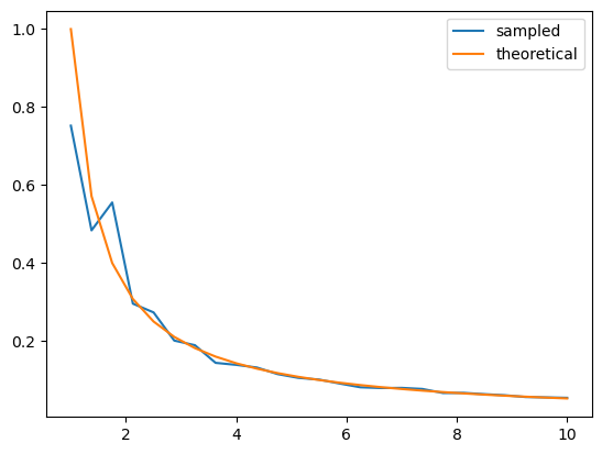
_images/285f033d774e0aed0b23c11839958e8f0be000708df439040014fc60b24487c4.png

In general, for a Pareto distribution, a higher tail index implies less weight in the right hand tail.

This means less extreme values for wealth and hence more equality.

More equality translates to a lower Gini index.

Exercise 29.2

The wealth process (29.1) is similar to a Kesten process.

This is because, according to (29.2), savings is constant for all wealth levels above \(\hat w\).

When savings is constant, the wealth process has the same quasi-linear structure as a Kesten process, with multiplicative and additive shocks.

The Kesten–Goldie theorem tells us that Kesten processes have Pareto tails under a range of parameterizations.

The theorem does not directly apply here, since savings is not always constant and since the multiplicative and additive terms in (29.1) are not IID.

At the same time, given the similarities, perhaps Pareto tails will arise.

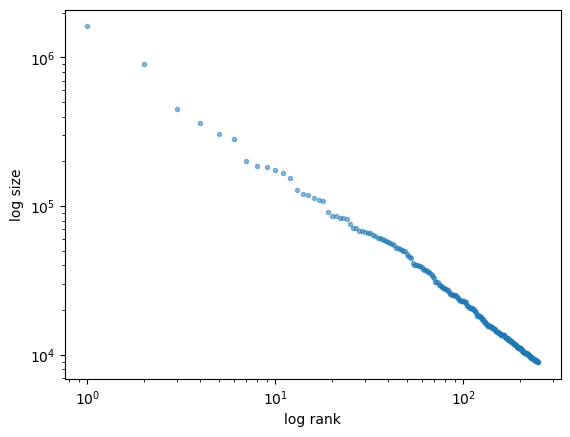
To test this, run a simulation that generates a cross-section of wealth and generate a rank-size plot.

If you like, you can use the function rank_size from the quantecon library (documentation here).

In viewing the plot, remember that Pareto tails generate a straight line. Is this what you see?

For sample size and initial conditions, use

num_households = 250_000
T = 500                                      # shift forward T periods
ψ_0 = np.full(num_households, wdy.y_mean)   # initial distribution
z_0 = wdy.z_mean

Solution to Exercise 29.2

First let’s generate the distribution:

num_households = 250_000
T = 500  # how far to shift forward in time
wdy = WealthDynamics()
ψ_0 = np.full(num_households, wdy.y_mean)
z_0 = wdy.z_mean

ψ_star = update_cross_section(wdy, ψ_0, shift_length=T)

Now let’s see the rank-size plot:

fig, ax = plt.subplots()

rank_data, size_data = qe.rank_size(ψ_star, c=0.001)
ax.loglog(rank_data, size_data, 'o', markersize=3.0, alpha=0.5)
ax.set_xlabel("log rank")
ax.set_ylabel("log size")

plt.show()

_images/a749774001908b38f547fc1a986138a0de436d62ecd6fd02e45a57ffade5562b.png

29. Wealth Distribution Dynamics#

29.1. Overview#

29.1.1. A Note on Assumptions#

29.2. Lorenz Curves and the Gini Coefficient#

29.2.1. Lorenz Curves#

29.2.2. The Gini Coefficient#

29.3. A Model of Wealth Dynamics#

29.4. Implementation#

29.5. Applications#

29.5.1. Time Series#

29.5.2. Inequality Measures#

29.6. Exercises#

29. Wealth Distribution Dynamics #

29.1. Overview #

29.2. Lorenz Curves and the Gini Coefficient #

29.3. A Model of Wealth Dynamics #

29.4. Implementation #

29.5. Applications #

29.6. Exercises #