38. Which Moments to Match?#
38.1. Overview#
Some structural economic models have the following two properties:
it is possible to compute an equilibrium and simulate it, given a known parameter vector
it is not possible to write down a likelihood function analytically
We can solve “the direct problem,” which maps a parameter vector into a probability distribution of the data.
We cannot use maximum likelihood to solve “the inverse problem,” which maps an observed data set into an estimate of the parameter vector.
Researchers with such models turn to the generalized method of moments of Hansen [1982] and compute the moments by simulation [Duffie and Singleton, 1993, McFadden, 1989, Pakes and Pollard, 1989].
They must decide which moments to match.
A. Ronald Gallant and George Tauchen studied this question in Gallant and Tauchen [1996].
They put two models on the table:
the economist’s structural model, indexed by a parameter vector \(\rho\), whose likelihood function cannot be written down
a distinct, descriptive auxiliary model, indexed by a parameter vector \(\theta\), whose likelihood function can be written down and maximized
The two parameter vectors usually differ in dimension and always differ in meaning.
\(\rho\) specifies the preferences, technologies, constraint sets and other features of the agents inside the structural model. The economist wants to learn \(\rho\).
\(\theta\) summarizes the observed data. Its components answer no economic question. The economist estimates \(\theta\) only as a step toward estimating \(\rho\).
structural model |
auxiliary model |
|
|---|---|---|
density |
\(p(y_t \mid x_t, \rho)\) |
\(f(y_t \mid x_t, \theta)\) |
parameter |
\(\rho \in \mathbb{R}^{k_\rho}\) |
\(\theta \in \mathbb{R}^{k_\theta}\) |
interpretation |
economic |
descriptive |
likelihood |
unavailable |
available |
role |
object of inference |
source of moment conditions |
Here \(x_t\) collects lagged values of \(y_t\), possibly the whole history.
In the stochastic volatility example below, \(\rho = (a, r_w, r_y)\) governs a latent log-volatility process, while \(\theta = (\mu, \omega, \alpha, \beta)\) holds the parameters of a GARCH(1,1) model.
No component of \(\theta\) corresponds to a component of \(\rho\).
Gallant and Tauchen’s method uses the scores associated with the likelihood function of the auxiliary model as the moment vector for GMM.
They fit \(\theta\) to the observed data once.
They then choose \(\rho\) so that, in data simulated from the structural model, the auxiliary score evaluated at that fitted \(\theta\) averages as close to zero as possible.
Note
Section Why the score is the right thing to match shows that the score moment conditions are the negative gradient of a Kullback-Leibler divergence. Statistical Divergence Measures and Likelihood Ratio Processes study properties of the KL divergence.
Gallant and Tauchen prove that if the auxiliary model nests the structural model, their estimator is as efficient as maximum likelihood.
They argue that if the auxiliary model closely approximates the distribution of the data, the estimator is nearly as efficient.
Practitioners call their method the efficient method of moments, or EMM.
Gallant and Tauchen [2010] surveys the method and its applications.
Let’s start with some imports.
import numpy as np
import matplotlib.pyplot as plt
from numba import jit
from scipy.optimize import minimize
from scipy.stats import chi2
38.2. The estimation problem#
A structural model is a sequence of probability densities for an observed process \(\{y_t\}\),
where \(x_t\) collects whatever the model conditions on, usually lagged values of \(y_t\).
We call \(\rho\) the structural parameter vector.
Nature generated the observed data \(\{\tilde y_t, \tilde x_t\}_{t=1}^n\) from \(\rho^0\).
Tildes mark observed data and statistics computed from them.
Hats mark simulated data and the final estimator \(\hat\rho_n\).
We assume two things about the structural model.
Simulation is feasible: given \(\rho\), we can generate a long artificial series \(\{\hat y_\tau, \hat x_\tau\}_{\tau=1}^N\).
The likelihood is unavailable: \(\prod_t p(\tilde y_t \mid \tilde x_t, \rho)\) has no expression that we can evaluate and maximize.
Gallant and Tauchen take a stationary Markov structural model as the leading case.
A single long simulation then suffices to compute any expectation under the model.
Their paper also covers independent cross-sectional data and processes whose laws of motion depend on \(t\).
38.3. The auxiliary model and its score#
An auxiliary model is a second sequence of densities for the same observed process,
We call \(\theta\) the auxiliary parameter vector.
Gallant and Tauchen call the auxiliary model the score generator.
Two properties make an auxiliary model useful.
Its density has an analytic expression, so we can write down its likelihood and differentiate it.
It describes the data well.
The first property is required.
Consistency requires only that the scores identify \(\rho\), as Exercise 38.1 and Exercise 38.3 show.
Section Choosing the score generator explains what a close fit buys.
A GARCH model of asset returns, a vector autoregression, and a Hermite series expansion of a conditional density all qualify.
The score of the auxiliary model is the derivative of its log density with respect to its own parameters,
The score is a \(k_\theta \times 1\) vector that we can evaluate at any \((y, x, \theta)\).
38.4. The estimator#
The estimator takes three steps.
Step 1. Projection. Fit the auxiliary model to the observed data by quasi-maximum likelihood,
This step uses the data and the auxiliary model alone, so it happens once, before any structural parameter is estimated.
Step 2. Moments by simulation. Define the moment function \(m(\rho, \theta)\) as the expectation under the structural model of the auxiliary score,
where \(p(x \mid \rho)\) is the stationary density of \(x_t\) under the structural model.
A long simulation approximates the double integral at \(\theta = \tilde\theta_n\),
The right side of (38.2) averages the auxiliary score over a long simulation from the structural model at \(\rho\).
Each evaluation requires a simulation and no optimization.
Step 3. GMM. Estimate \(\rho\) by making the moment vector as close to zero as the GMM metric allows,
where
The weighting matrix (38.4) is the outer product of the auxiliary scores at the data.
It estimates \(\mathcal{I}^0\), the asymptotic variance of \(n^{-1/2} \sum_{t=1}^n s(\tilde y_t, \tilde x_t, \theta^0)\), where \(\theta^0\) is the probability limit of \(\tilde\theta_n\).
It depends on the auxiliary model and the data alone.
The outer product is a valid estimate when the scores are serially uncorrelated.
An auxiliary model that describes the conditional distribution of the data correctly delivers serially uncorrelated scores.
Gaussian quasi-maximum likelihood scores are also serially uncorrelated when the auxiliary model specifies the conditional mean and variance correctly [Bollerslev and Wooldridge, 1992].
Otherwise Gallant and Tauchen recommend a heteroskedasticity and autocorrelation consistent estimate with Parzen weights [Gallant, 1987], and they cite Andrews [1991] for alternatives.
Exercise 38.4 shows how far the outer product can understate \(\mathcal{I}^0\) when the scores are serially correlated.
A researcher computes either estimate once, before the search over \(\rho\) begins.
GMM usually requires a preliminary estimate of the structural parameters to form an efficient weighting matrix, and with either of these estimates that requirement disappears.
The order condition for identification is \(k_\theta \ge k_\rho\).
The order condition is necessary but not sufficient, and Exercise 38.3 constructs a failure.
38.5. Why the score is the right thing to match#
Statistical Divergence Measures shows that maximum likelihood minimizes the KL divergence from the empirical distribution of the data to the parametric model.
Step 1 projects the data onto the auxiliary family by minimizing KL divergence.
For each \(\rho\), define the pseudo-true value
the point in the auxiliary family closest to the structural model at \(\rho\) [White, 1982] [1].
The function \(\theta^0(\cdot)\) maps structural parameters into auxiliary parameters.
As \(n\) grows, \(\tilde\theta_n\) converges to \(\theta^0 = \theta^0(\rho^0)\).
Now differentiate the divergence with respect to \(\theta\):
The moment function (38.1) is the negative gradient of a Kullback-Leibler divergence.
Setting \(m(\rho, \theta) = 0\) states the first-order condition for a KL projection.
The estimator (38.3) searches for the structural parameter whose KL projection onto the auxiliary family lands where the data’s projection landed, or as close as the GMM metric allows when \(k_\theta > k_\rho\).
This reading explains why the structural model need not nest inside the auxiliary model.
At \(\rho = \rho^0\) the structural model generated the data, the two projections coincide, and \(m(\rho^0, \theta^0) = 0\).
Exercise 38.1 asks you to verify this chain of reasoning.
38.6. Efficiency#
Consistency and asymptotic normality hold under weak regularity conditions,
which is Theorem 1 of Gallant and Tauchen [1996].
Here \(\mathcal{I}^0\) is the variance of the auxiliary score that \(\tilde{\mathcal{I}}_n\) in (38.4) estimates.
The formula assumes that the weighting matrix converges to \((\mathcal{I}^0)^{-1}\), as \((\tilde{\mathcal{I}}_n)^{-1}\) does when \(\tilde{\mathcal{I}}_n\) estimates \(\mathcal{I}^0\) consistently.
With any other limiting weighting matrix \(W\), the asymptotic variance takes the sandwich form
Exercise 38.4 uses it.
Gallant and Tauchen assume that \(N\) is large enough to make simulation error negligible, so the formula treats \(m\) as computed exactly.
A simulation of length \(N\) adds independent noise to \(m\) and multiplies the asymptotic variance of \(\sqrt{n}\, m\), and hence of \(\hat\rho_n\), by \(1 + n/N\).
Gallant and Tauchen say that the structural model is smoothly embedded within the auxiliary model when a twice continuously differentiable map \(g\) carries structural parameters into auxiliary parameters,
Smooth embedding says that the auxiliary model nests the structural model.
In general \(p(\cdot \mid \rho)\) lies outside the auxiliary family, and no \(g\) satisfies this equation.
The function \(\theta^0(\rho)\) always exists.
Under smooth embedding \(\theta^0(\rho) = g(\rho)\).
Write \(G^0 = \partial g(\rho^0) / \partial \rho^\top\).
Their Theorem 2 states that smooth embedding implies
which is the asymptotic distribution of the maximum likelihood estimator of \(\rho\).
The proof turns on the identity \(M^0 = \mathcal{I}^0 G^0\), which converts the GMM variance into the ML variance.
The estimator attains maximum likelihood efficiency without the structural likelihood.
Smooth embedding is a strong assumption, and consistency and asymptotic normality do not require it.
Gallant and Tauchen argue that an auxiliary model that approximates the distribution of the data closely without nesting the structural model delivers an estimator that is nearly fully efficient.
Gallant and Tauchen read this as instruction about how to choose the auxiliary model: make it fit.
38.7. Comparison with matching the auxiliary parameters#
Indirect inference names the class of estimators that compare observed and simulated data through an auxiliary model.
Gourieroux et al. [1993] and Smith [1993] match the auxiliary parameters.
Gourieroux et al. [1993] call \(\theta^0(\rho)\) the binding function.
Their estimator is
for a weighting matrix \(\Omega\).
Under smooth embedding \(\theta^0 = g\), and the choice \(\Omega = \mathcal{I}^0\) yields the minimum chi-square estimator, which is as efficient as maximum likelihood.
The binding function is unavailable whenever the structural likelihood is unavailable, so a practitioner replaces \(\theta^0(\rho)\) by the average of auxiliary estimates computed on \(H\) simulated data sets.
That replacement is expensive.
Each trial value of \(\rho\) requires \(H\) separate maximizations of the auxiliary likelihood, one per simulated data set.
The score-based estimator requires exactly one maximization of the auxiliary likelihood, in Step 1, and never repeats it.
With suitably chosen weighting matrices, the parameter-based and score-based estimators are asymptotically equivalent [Gourieroux et al., 1993].
The advantage of matching scores is computational.
Finite-sample behavior can differ.
Duffee and Stanton [2008] study highly persistent Gaussian autoregressions and find that score matching yields confidence intervals that are wider than those of parameter matching yet less likely to cover the true value.
They trace the problem to the large role that the population variance plays in the score moment conditions.
38.8. Choosing the score generator#
A model known to describe the data accurately should be the auxiliary model.
Lacking one, Gallant and Tauchen recommend two general purpose families.
The seminonparametric or SNP density of Gallant and Nychka [1987] and Gallant and Tauchen [1989] multiplies a Gaussian density by a squared Hermite polynomial whose coefficients depend on lagged values.
Tuning parameters nest an IID Gaussian, a Gaussian VAR, Gaussian ARCH and GARCH, and fully nonlinear nonparametric specifications, so a specification search selects the auxiliary model from the data [Gallant and Tauchen, 2010].
The neural net score approximates any nonlinear autoregression, including deterministic chaos.
Both families are series expansions, so adding terms drives the approximation error to zero.
Adding terms also drives the conditional mean of the score toward zero, so the scores approach martingale differences.
The outer product (38.4) then estimates \(\mathcal{I}^0\) accurately, and the weighting matrix needs no correction for serial correlation.
A close fit therefore buys two things: near efficiency and a valid outer-product weighting matrix.
Exercise 38.4 shows what happens with a score generator that lacks the second.
The number of terms governs a trade-off between bias and variance.
More terms reduce the approximation error of the auxiliary model and raise the sampling variance of \(\tilde\theta_n\).
Gallant and Tauchen warn against taking too many terms and then claiming that standard asymptotics apply.
38.9. A first example: an AR(1) inside an AR(2)#
An example in which we can compute the maximum likelihood estimator lets us check Theorem 2.
Take as the structural model a Gaussian first-order autoregression,
with \(\rho = (\rho_1, \sigma)^\top\).
Take as the auxiliary model a Gaussian second-order autoregression,
with \(\theta = (\theta_1, \theta_2, \varsigma)^\top\).
The AR(2) nests the AR(1) through \(g(\rho_1, \sigma) = (\rho_1, 0, \sigma)\), so the structural model is smoothly embedded and \(k_\theta = 3\) exceeds \(k_\rho = 2\).
The components \(\theta_1\) and \(\rho_1\) share an interpretation only because the AR(2) nests the AR(1).
Theorem 2 predicts that our estimator and the maximum likelihood estimator have the same asymptotic distribution, up to the simulation factor \(1 + n/N\).
Writing \(u_t = y_t - \theta_1 y_{t-1} - \theta_2 y_{t-2}\), the auxiliary score is
@jit(nopython=True)
def simulate_ar1(ρ1, σ, ε):
    "Simulate the structural AR(1) from a fixed array of shocks ε."
    n = ε.size
    y = np.empty(n)
    y[0] = σ * ε[0] / np.sqrt(1 - ρ1**2)
    for t in range(1, n):
        y[t] = ρ1 * y[t-1] + σ * ε[t]
    return y

def ar2_scores(θ, y):
    "Per-observation scores of the Gaussian AR(2) auxiliary model."
    θ1, θ2, ς = θ
    yt, y1, y2 = y[2:], y[1:-1], y[:-2]
    u = yt - θ1 * y1 - θ2 * y2
    return np.column_stack([u * y1 / ς**2, u * y2 / ς**2, -1/ς + u**2 / ς**3])

def ar2_qmle(y):
    "Quasi-maximum likelihood estimates of the AR(2), available in closed form."
    X = np.column_stack([y[1:-1], y[:-2]])
    b = np.linalg.lstsq(X, y[2:], rcond=None)[0]
    ς = np.sqrt(np.mean((y[2:] - X @ b)**2))
    return np.array([b[0], b[1], ς])
Let’s generate data from the structural model and compute the conditional maximum likelihood estimator, which for this model is least squares.
rng = np.random.default_rng(0)
T, ρ1_0, σ_0 = 1000, 0.8, 1.0
y_data = simulate_ar1(ρ1_0, σ_0, rng.standard_normal(T))

X1 = y_data[:-1]
ρ1_mle = float(X1 @ y_data[1:] / (X1 @ X1))
σ_mle = float(np.sqrt(np.mean((y_data[1:] - ρ1_mle * X1)**2)))
print(f"maximum likelihood:  ρ1 = {ρ1_mle:.4f}   σ = {σ_mle:.4f}")
maximum likelihood: ρ1 = 0.8022 σ = 0.9784
Step 1 fits the auxiliary model and forms the weighting matrix.
θ_tilde = ar2_qmle(y_data)
S = ar2_scores(θ_tilde, y_data)
I_tilde = S.T @ S / S.shape[0]
W = np.linalg.inv(I_tilde)

print(f"auxiliary QMLE: θ1 = {θ_tilde[0]:.4f}, θ2 = {θ_tilde[1]:.4f}, ς = {θ_tilde[2]:.4f}")
auxiliary QMLE: θ1 = 0.8083, θ2 = -0.0075, ς = 0.9789
The estimate of \(\theta_2\) sits near zero, as the nesting map \(g\) anticipates.
Steps 2 and 3 simulate and minimize.
We draw the shocks \(\epsilon\) once and reuse them at every trial value of \(\rho\).
We call them common random numbers, and a figure below shows their effect on the criterion.
N = 20_000
ε_sim = rng.standard_normal(N)      # common random numbers

def moments_ar1(ρ):
    "Expectation under the structural model of the auxiliary score."
    y_sim = simulate_ar1(ρ[0], ρ[1], ε_sim)
    return ar2_scores(θ_tilde, y_sim).mean(axis=0)

def criterion_ar1(ρ):
    if not (abs(ρ[0]) < 0.999 and ρ[1] > 1e-6):
        return 1e10
    m = moments_ar1(ρ)
    return float(m @ W @ m)

res = minimize(criterion_ar1, np.array([0.5, 1.5]), method='Nelder-Mead',
               options=dict(xatol=1e-6, fatol=1e-12, maxiter=2000))

print(f"true values:         ρ1 = {ρ1_0:.4f}   σ = {σ_0:.4f}")
print(f"maximum likelihood:  ρ1 = {ρ1_mle:.4f}   σ = {σ_mle:.4f}")
print(f"score matching:      ρ1 = {res.x[0]:.4f}   σ = {res.x[1]:.4f}")
true values:         ρ1 = 0.8000   σ = 1.0000
maximum likelihood:  ρ1 = 0.8022   σ = 0.9784
score matching:      ρ1 = 0.8009   σ = 0.9830
The two sets of estimates nearly coincide, differing in the third decimal place.
The next figure evaluates the criterion on a grid of \(\rho_1\) values with \(\sigma\) held at its estimate.
One curve uses the common random numbers ε_sim, and the other draws fresh shocks at each grid point.
rng_fresh = np.random.default_rng(1)
ρ1_grid = np.linspace(0.77, 0.83, 61)
σ_hat = res.x[1]

def criterion_fresh(ρ):
    "The criterion with a fresh draw of shocks at each evaluation."
    y_sim = simulate_ar1(ρ[0], ρ[1], rng_fresh.standard_normal(N))
    m = ar2_scores(θ_tilde, y_sim).mean(axis=0)
    return float(m @ W @ m)

crn = [criterion_ar1(np.array([r1, σ_hat])) for r1 in ρ1_grid]
fresh = [criterion_fresh(np.array([r1, σ_hat])) for r1 in ρ1_grid]

fig, ax = plt.subplots()
ax.plot(ρ1_grid, crn, lw=2, label='common random numbers')
ax.plot(ρ1_grid, fresh, lw=2, label='fresh shocks at each point')
ax.set_xlabel(r'$\rho_1$')
ax.set_ylabel('criterion')
ax.legend()
plt.show()
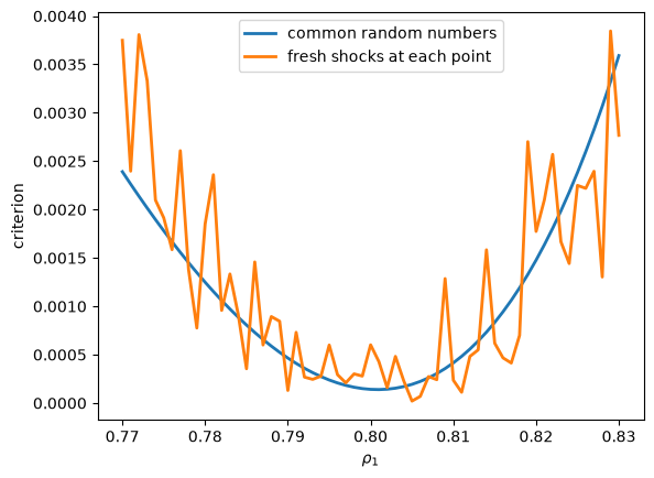
Fig. 38.1 Criterion with common and fresh shocks#
Fresh shocks make the criterion jagged, with many local minima.
Common random numbers make it a smooth function of \(\rho_1\) with a single minimum.
The minimized criterion tests the \(k_\theta - k_\rho = 1\) overidentifying restriction that the structural model places on the auxiliary model.
Under correct specification, \(n\) times the minimized criterion, divided by the simulation factor \(1 + n/N\), is asymptotically distributed as \(\chi^2(k_\theta - k_\rho)\) [2].
The code writes the sample size \(n\) as T.
J = T * criterion_ar1(res.x) / (1 + T / N)
df = 3 - 2
print(f"J = {J:.3f},  χ²({df}) 5% critical value = {chi2.ppf(0.95, df):.3f}")
J = 0.133, χ²(1) 5% critical value = 3.841
Theorem 1 delivers standard errors.
We compute \(M^0\) by central differences of the simulated moment vector, which common random numbers make smooth in \(\rho\), and we multiply the variance by the simulation factor \(1 + n/N\).
For the AR(1), the maximum likelihood standard errors are \(\sqrt{(1 - \rho_1^2)/n}\) for \(\rho_1\) and \(\sigma / \sqrt{2n}\) for \(\sigma\).
def jacobian(moments, ρ, h=1e-4):
    "Central-difference Jacobian of a moment function with respect to ρ."
    cols = []
    for j in range(ρ.size):
        e = np.zeros(ρ.size)
        e[j] = h * max(1.0, abs(ρ[j]))
        cols.append((moments(ρ + e) - moments(ρ - e)) / (2 * e[j]))
    return np.column_stack(cols)

def std_errors(moments, ρ, W, n, N):
    "Asymptotic standard errors from Theorem 1, including the simulation factor."
    M = jacobian(moments, ρ)
    V = np.linalg.inv(M.T @ W @ M) * (1 + n / N) / n
    return np.sqrt(np.diag(V))

se_emm = std_errors(moments_ar1, res.x, W, T, N)
se_mle = np.array([np.sqrt((1 - ρ1_mle**2) / T), σ_mle / np.sqrt(2 * T)])

print(f"{'':20}{'se ρ1':>10}{'se σ':>10}")
print(f"{'maximum likelihood':20}{se_mle[0]:10.4f}{se_mle[1]:10.4f}")
print(f"{'score matching':20}{se_emm[0]:10.4f}{se_emm[1]:10.4f}")

e_data = y_data[1:] - ρ1_mle * y_data[:-1]
kurt_e = ((e_data - e_data.mean())**4).mean() / e_data.var()**2
print(f"\nkurtosis of the residuals = {kurt_e:.2f}")
                         se ρ1      se σ
maximum likelihood      0.0189    0.0219
score matching          0.0188    0.0241

kurtosis of the residuals = 3.29
The two standard errors for \(\rho_1\) agree to three decimal places.
The score matching standard error for \(\sigma\) exceeds the maximum likelihood one by about 10 percent.
The simulation factor \(1 + n/N = 1.05\) accounts for about 2.5 percent.
The weighting matrix \(\tilde{\mathcal{I}}_n\) accounts for the rest: it estimates the variance of the \(\sigma\) score from the sample fourth moment of the residuals, whose kurtosis is 3.3 in this sample and 3 in the population.
Exercise 38.2 asks you to compare the sampling distributions of the two estimators.
38.10. A second example: stochastic volatility#
Now we turn to a model whose likelihood function is intractable.
Section 4.2 of Gallant and Tauchen [1996] discusses a stochastic volatility model whose mean equation also contains an intercept and a lagged return.
We drop those two terms and study
with \(z_t\) and \(\eta_t\) independent standard normals and \(\rho = (a, r_w, r_y)^\top\).
The observed return \(y_t\) has a volatility \(\exp(w_t) r_y\) driven by a latent autoregression \(w_t\).
Writing the likelihood of \(\{y_t\}_{t=1}^n\) requires integrating the latent volatility path out of an \(n\)-dimensional integral,
which no analytic expression evaluates.
Simulating the model takes two lines of code.
The model generates fat tails and persistent volatility.
Gallant et al. [1997] fit the full model and extensions of it to 16,127 daily observations on the Standard and Poor’s composite index, using SNP score generators.
Section 4.1 of Gallant and Tauchen [1996] notes that ARCH and GARCH models fit returns data well.
We choose as the auxiliary model a Gaussian GARCH(1,1),
with \(\theta = (\mu, \omega, \alpha, \beta)^\top\) and \(\nu_t \sim N(0,1)\).
The GARCH conditional density depends on the entire past of \(y_t\) through the recursion for \(\sigma_t^2\), so here \(x_t\) is the whole history.
Gallant and Tauchen call such a score generator non-Markov.
The structural parameters \((a, r_w, r_y)\) describe a latent log-volatility process; the auxiliary parameters \((\mu, \omega, \alpha, \beta)\) describe a conditional variance recursion in observed returns.
The auxiliary model needs no economic interpretation.
Its credential is a good fit to the data.
We differentiate the GARCH log density numerically.
Numerical differentiation keeps the method general: an auxiliary model need only support evaluation of its log likelihood.
The code fits the GARCH model in the unconstrained coordinates \((\mu, \log \omega, \operatorname{logit} \alpha, \operatorname{logit} \beta)\).
The scores, the weighting matrix, and the moment vector all refer to those coordinates.
The reparameterization changes neither \(\hat\rho_n\) nor the test statistic.
It multiplies the score by a fixed invertible matrix, and the criterion (38.3) is invariant to that transformation.
@jit(nopython=True)
def simulate_sv(a, r_w, r_y, z, η):
    "Simulate the structural stochastic volatility model."
    n = z.size
    y = np.empty(n)
    w = r_w * η[0] / np.sqrt(1.0 - a * a)
    y[0] = np.exp(w) * r_y * z[0]
    for t in range(1, n):
        w = a * w + r_w * η[t]
        y[t] = np.exp(w) * r_y * z[t]
    return y

@jit(nopython=True)
def garch_ll(μ, ω, α, β, y):
    "Per-observation log densities of the Gaussian GARCH(1,1) auxiliary model."
    n = y.size
    ll = np.empty(n)
    s2 = ω / max(1e-8, 1.0 - α - β)
    for t in range(n):
        u = y[t] - μ
        ll[t] = -0.5 * (np.log(2 * np.pi) + np.log(s2) + u * u / s2)
        s2 = ω + α * u * u + β * s2
    return ll

def unpack(θ):
    "Map unconstrained parameters to ω > 0 and α, β in (0, 1)."
    μ, lω, lα, lβ = θ
    return μ, np.exp(lω), 1 / (1 + np.exp(-lα)), 1 / (1 + np.exp(-lβ))

def garch_negll(θ, y):
    μ, ω, α, β = unpack(θ)
    if α + β > 0.999:
        return 1e10
    return -garch_ll(μ, ω, α, β, y).sum()

def garch_scores(θ, y):
    "Per-observation auxiliary scores by central differences."
    p, n = θ.size, y.size
    S = np.empty((n, p))
    for j in range(p):
        h = 1e-5 * max(1.0, abs(θ[j]))
        θp, θm = θ.copy(), θ.copy()
        θp[j] += h
        θm[j] -= h
        S[:, j] = (garch_ll(*unpack(θp), y) - garch_ll(*unpack(θm), y)) / (2 * h)
    return S
Section 4.2 reports no parameter values, so we choose our own.
Let’s generate a long return series from the structural model.
rng = np.random.default_rng(5)
T = 2000
a_0, r_w0, r_y0 = 0.80, 0.20, 0.65
y_sv = simulate_sv(a_0, r_w0, r_y0, rng.standard_normal(T), rng.standard_normal(T))

kurt = ((y_sv - y_sv.mean())**4).mean() / y_sv.var()**2
print(f"standard deviation = {y_sv.std():.3f},  kurtosis = {kurt:.2f}")
standard deviation = 0.738, kurtosis = 3.93
The population kurtosis of \(y_t\) is \(3 \exp\bigl( 4 r_w^2 / (1 - a^2) \bigr) = 4.7\) at these parameter values, above the Gaussian value of 3.
The sample kurtosis understates it, as sample kurtoses of heavy-tailed series often do.
fig, ax = plt.subplots()
ax.plot(y_sv, lw=0.6)
ax.set_xlabel('$t$')
ax.set_ylabel('$y_t$')
plt.show()
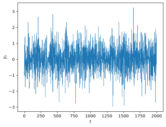
Fig. 38.2 Simulated returns from the SV model#
Step 1 fits the GARCH auxiliary model to these data.
θ_start = np.array([0.0, np.log(0.05), -2.0, 1.5])
r = minimize(garch_negll, θ_start, args=(y_sv,), method='Nelder-Mead',
             options=dict(maxiter=8000, xatol=1e-8, fatol=1e-8))
θ_sv = r.x
μ_h, ω_h, α_h, β_h = unpack(θ_sv)
print(f"auxiliary GARCH QMLE: μ = {μ_h:.4f}, ω = {ω_h:.4f}, "
      f"α = {α_h:.4f}, β = {β_h:.4f}   (α + β = {α_h + β_h:.4f})")

S_sv = garch_scores(θ_sv, y_sv)
W_sv = np.linalg.inv(S_sv.T @ S_sv / T)
auxiliary GARCH QMLE: μ = 0.0150, ω = 0.0922, α = 0.1209, β = 0.7127 (α + β = 0.8337)
An \(\alpha + \beta\) of 0.83 records the persistence of volatility that the auxiliary model reads off the data.
Steps 2 and 3 estimate the three structural parameters.
We search over unconstrained coordinates and reuse one pair of shock arrays throughout.
N = 50_000
z_sim, η_sim = rng.standard_normal(N), rng.standard_normal(N)

def moments_sv(ρ):
    y_s = simulate_sv(ρ[0], ρ[1], ρ[2], z_sim, η_sim)
    return garch_scores(θ_sv, y_s).mean(axis=0)

def to_ρ(u):
    "Map unconstrained coordinates to a in (0,1) and r_w, r_y > 0."
    return np.array([1 / (1 + np.exp(-u[0])), np.exp(u[1]), np.exp(u[2])])

def criterion_sv(u):
    if np.max(np.abs(u)) > 25:
        return 1e10
    m = moments_sv(to_ρ(u))
    return float(m @ W_sv @ m)

u_0 = np.array([np.log(0.6 / 0.4), np.log(0.3), np.log(0.5)])
res_sv = minimize(criterion_sv, u_0, method='Nelder-Mead',
                  options=dict(maxiter=400, xatol=1e-4, fatol=1e-10))
ρ_hat = to_ρ(res_sv.x)
Theorem 1 delivers standard errors.
se_sv = std_errors(moments_sv, ρ_hat, W_sv, T, N)

print(f"{'':17}{'a':>9}{'r_w':>9}{'r_y':>9}")
print(f"{'true values':17}{a_0:9.4f}{r_w0:9.4f}{r_y0:9.4f}")
print(f"{'score matching':17}" + "".join(f"{x:9.4f}" for x in ρ_hat))
print(f"{'standard errors':17}" + "".join(f"{x:9.4f}" for x in se_sv))
                         a      r_w      r_y
true values         0.8000   0.2000   0.6500
score matching      0.8447   0.1794   0.6700
standard errors     0.0404   0.0372   0.0244
The estimator locates all three parameters of a model whose likelihood function we never wrote down.
Each estimate lies within about one standard error of its true value.
The data pin down the scale \(r_y\) most precisely.
38.11. Testing the structural model#
The auxiliary model has four parameters and the structural model has three, so one overidentifying restriction remains to be tested.
J_sv = T * criterion_sv(res_sv.x) / (1 + T / N)
df_sv = 4 - 3
print(f"J = {J_sv:.3f},  χ²({df_sv}) 5% critical value = {chi2.ppf(0.95, df_sv):.3f}")
J = 0.606, χ²(1) 5% critical value = 3.841
The data give the structural model no trouble, as they should, because the structural model generated them.
A misspecified structural model fares differently.
Let’s impose \(r_w = 0\), which shuts down stochastic volatility and leaves a Gaussian white noise with one free parameter.
def moments_const_vol(v):
    "Moments of the constant volatility model r_w = 0, with v = log r_y; a has no effect."
    return moments_sv(np.array([0.5, 1e-8, np.exp(v[0])]))

def criterion_const_vol(v):
    m = moments_const_vol(v)
    return float(m @ W_sv @ m)

r_cv = minimize(criterion_const_vol, np.array([0.0]), method='Nelder-Mead',
                options=dict(maxiter=200, xatol=1e-6))
J_cv = T * criterion_const_vol(r_cv.x) / (1 + T / N)
df_cv = 4 - 1
print(f"constant volatility model: J = {J_cv:.1f}, "
      f"χ²({df_cv}) 5% critical value = {chi2.ppf(0.95, df_cv):.3f}")
constant volatility model: J = 21.0, χ²(3) 5% critical value = 7.815
The test rejects the restricted model at the 1% level [3].
Gallant and Tauchen emphasize this second use of the machinery.
An auxiliary model that approximates the data well makes the test powerful against structural model error, and the individual score components say which features of the data a rejected model fails to match.
Gallant and Tauchen’s quasi-t-ratios divide each component of \(\sqrt{n}\, m(\hat\rho_n, \tilde\theta_n)\) by its standard error.
The asymptotic variance of \(\sqrt{n}\, m(\hat\rho_n, \tilde\theta_n)\) is
Estimating \(\rho\) removes the variance in the directions that the columns of \(M^0\) span.
The unconstrained coordinates transform each GARCH parameter separately through an increasing function.
The t-ratios are therefore the same as in the coordinates \((\mu, \omega, \alpha, \beta)\).
I_sv = S_sv.T @ S_sv / T
M_cv = jacobian(moments_const_vol, r_cv.x)
V_cv = (I_sv - M_cv @ np.linalg.inv(M_cv.T @ W_sv @ M_cv) @ M_cv.T) * (1 + T / N)
t_cv = np.sqrt(T) * moments_const_vol(r_cv.x) / np.sqrt(np.diag(V_cv))

for name, t in zip(['μ', 'ω', 'α', 'β'], t_cv):
    print(f"{name:>4}: {t:6.2f}")
   μ:  -0.75
   ω:  -3.04
   α:  -3.95
   β:  -2.79
The components for \(\omega\), \(\alpha\) and \(\beta\), which govern the conditional variance, carry the rejection.
The \(\mu\) component does not.
Each negative sign says that, holding the other auxiliary parameters fixed, data from the constant volatility model would pull that parameter below the value that the observed data choose.
The constant volatility model matches the mean of returns and fails to reproduce the dependence of today’s variance on yesterday’s squared return.
Gallant et al. [1997] use the score vector of a rejected stochastic volatility model to diagnose its defects, and they then repair the model by thickening the tails of \(z_t\) and lengthening the memory of the volatility equation.
38.12. Applications#
Gallant and Tauchen [2010] collects applications of the method to continuous-time models in finance.
Andersen et al. [2002] estimate stochastic volatility diffusions for the Standard and Poor’s 500 index and reject them, and jump diffusions pass the same tests.
Other applications fit multifactor stochastic volatility models, term structure models of interest rates, and exchange rate models.
Bansal et al. [1995] fit a two-country general equilibrium monetary model to high-frequency currency market data, and Gallant and Tauchen [1996] propose fitting a one-sector stochastic growth model to consumption and stock returns.
Empirical auction models form another class of applications.
Game theory delivers the density of the winning bid under independent private values, and that density has a tractable form only for special valuation distributions.
Simulating from it is easy for any valuation distribution, so score matching brings all of the restrictions of the theory to bear.
38.13. Recovering the latent state#
Having estimated \(\rho\), a researcher often wants the latent state, such as the volatility path behind a return series.
Reprojection recovers it [Gallant and Tauchen, 2010].
Simulate a long path of states and observables at \(\hat\rho_n\), calibrate inside the simulation the conditional distribution of the latent state given current and lagged observables, then evaluate those calibrated functions at the observed data.
Reprojection is a simulation-based nonlinear filter.
38.15. Exercises#
Exercise 38.1
Let the structural model at \(\rho\) have density \(p(\cdot \mid \rho)\) and let the auxiliary family be \(\{f(\cdot \mid \theta) : \theta \in \Theta\}\).
a. Show that
where \(m(\rho,\theta) = \mathbb{E}_{p(\cdot \mid \rho)} \bigl[ \partial \ln f(\cdot \mid \theta) / \partial\theta \bigr]\).
b. Conclude that the pseudo-true value \(\theta^0(\rho)\) satisfies \(m\bigl(\rho, \theta^0(\rho)\bigr) = 0\).
c. Explain why \(m(\rho^0, \theta^0) = 0\), and why the structural model does not need to nest inside the auxiliary family for this to hold.
Solution
For part a, write the divergence as
The first term does not involve \(\theta\).
Differentiating the second term under the integral sign gives
For part b, the pseudo-true value minimizes the divergence over \(\theta\).
An interior minimum sets the gradient to zero, so \(m\bigl(\rho, \theta^0(\rho)\bigr) = 0\).
For part c, nature generated the data from \(\rho^0\), so the quasi-maximum likelihood estimator \(\tilde\theta_n\) converges to \(\theta^0 = \theta^0(\rho^0)\), the KL projection of the true data generating process.
Part b evaluated at \(\rho = \rho^0\) then gives \(m(\rho^0, \theta^0) = 0\).
Nesting plays no role in this argument.
The pseudo-true value is defined as a projection whether or not the divergence at its minimum is zero, and the divergence is zero only in the nested case.
A misspecified auxiliary model still delivers valid moment conditions.
It costs efficiency.
It preserves consistency.
Exercise 38.2
Theorem 2 of Gallant and Tauchen [1996] says that the score matching estimator and the maximum likelihood estimator have the same asymptotic distribution when the structural model is smoothly embedded within the auxiliary model and simulation error is negligible.
Check this claim by Monte Carlo in the AR(1) and AR(2) example.
Generate 60 independent samples of length \(T = 500\) from the structural AR(1) with \(\rho_1 = 0.8\) and \(\sigma = 1\).
For each sample compute both estimators, then compare their means, their standard deviations, and the correlation between them across replications.
Compare the Monte Carlo standard deviations with the asymptotic standard deviations that Theorem 2 delivers.
Solution
T_mc, N_mc, R = 500, 20_000, 60
rng_mc = np.random.default_rng(7)
ε_mc = rng_mc.standard_normal(N_mc)        # common random numbers

def emm_estimate(y, ε):
    "Score matching estimate of (ρ1, σ) from the sample y with the shock array ε."
    θ_r = ar2_qmle(y)
    S_r = ar2_scores(θ_r, y)
    W_r = np.linalg.inv(S_r.T @ S_r / S_r.shape[0])

    def crit_r(ρ):
        if not (abs(ρ[0]) < 0.999 and ρ[1] > 1e-6):
            return 1e10
        m = ar2_scores(θ_r, simulate_ar1(ρ[0], ρ[1], ε)).mean(axis=0)
        return float(m @ W_r @ m)

    return minimize(crit_r, np.array([0.5, 1.2]), method='Nelder-Mead',
                    options=dict(xatol=1e-6, fatol=1e-12)).x

samples = [simulate_ar1(ρ1_0, σ_0, rng_mc.standard_normal(T_mc)) for _ in range(R)]
mle_draws = np.empty((R, 2))
emm_draws = np.empty((R, 2))

for r_, y_r in enumerate(samples):
    X_r = y_r[:-1]
    ρ_m = float(X_r @ y_r[1:] / (X_r @ X_r))
    σ_m = float(np.sqrt(np.mean((y_r[1:] - ρ_m * X_r)**2)))
    mle_draws[r_] = [ρ_m, σ_m]
    emm_draws[r_] = emm_estimate(y_r, ε_mc)

print(f"{'':20}{'mean ρ1':>10}{'sd ρ1':>10}{'mean σ':>10}{'sd σ':>10}")
print(f"{'maximum likelihood':20}{mle_draws[:,0].mean():10.4f}{mle_draws[:,0].std():10.4f}"
      f"{mle_draws[:,1].mean():10.4f}{mle_draws[:,1].std():10.4f}")
print(f"{'score matching':20}{emm_draws[:,0].mean():10.4f}{emm_draws[:,0].std():10.4f}"
      f"{emm_draws[:,1].mean():10.4f}{emm_draws[:,1].std():10.4f}")
sd_theory = [np.sqrt((1 - ρ1_0**2) / T_mc), σ_0 / np.sqrt(2 * T_mc)]
print(f"{'asymptotic theory':20}{ρ1_0:10.4f}{sd_theory[0]:10.4f}"
      f"{σ_0:10.4f}{sd_theory[1]:10.4f}")
print(f"\ncorrelation across replications: ρ1 "
      f"{np.corrcoef(emm_draws[:,0], mle_draws[:,0])[0,1]:.4f}, "
      f"σ {np.corrcoef(emm_draws[:,1], mle_draws[:,1])[0,1]:.4f}")
                       mean ρ1     sd ρ1    mean σ      sd σ
maximum likelihood      0.8038    0.0274    0.9981    0.0315
score matching          0.7991    0.0275    1.0015    0.0321
asymptotic theory       0.8000    0.0268    1.0000    0.0316

correlation across replications: ρ1 0.9976, σ 0.9748
fig, axes = plt.subplots(1, 2)
for j, name in enumerate([r'$\rho_1$', r'$\sigma$']):
    axes[j].scatter(mle_draws[:, j], emm_draws[:, j], s=18)
    lo = min(mle_draws[:, j].min(), emm_draws[:, j].min())
    hi = max(mle_draws[:, j].max(), emm_draws[:, j].max())
    axes[j].plot([lo, hi], [lo, hi], 'k--', lw=1)
    axes[j].set_xlabel(f'maximum likelihood, {name}')
    axes[j].set_ylabel(f'score matching, {name}')
plt.tight_layout()
plt.show()
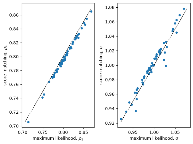
The two estimators have nearly identical standard deviations.
Both standard deviations are close to the asymptotic values \(\sqrt{(1 - \rho_1^2)/T}\) and \(\sigma / \sqrt{2T}\) that Theorem 2 delivers.
The simulation factor \(1 + T/N\) raises the score matching values by about 1 percent.
The correlation between the two estimators across replications sits very close to one, and the scatter plots hug the 45 degree line.
The two estimators are nearly the same random variable in each sample.
The means of the two estimators of \(\rho_1\) differ by about 0.005.
Every replication shares the shock array ε_mc, so its simulation error shifts all 60 score matching estimates together.
The next cell repeats the score matching estimates of \(\rho_1\) with three other shock arrays.
gap = (emm_draws[:, 0] - mle_draws[:, 0]).mean()
print(f"shock array ε_mc:       mean gap in ρ1 = {gap:7.4f}")
for seed in (100, 101, 102):
    ε_alt = np.random.default_rng(seed).standard_normal(N_mc)
    ρ1_alt = np.array([emm_estimate(y_r, ε_alt)[0] for y_r in samples])
    gap = (ρ1_alt - mle_draws[:, 0]).mean()
    print(f"shock array seed {seed}:  mean gap in ρ1 = {gap:7.4f}")
shock array ε_mc:       mean gap in ρ1 = -0.0047
shock array seed 100:  mean gap in ρ1 =  0.0013
shock array seed 101:  mean gap in ρ1 =  0.0041
shock array seed 102:  mean gap in ρ1 =  0.0004
The gap changes sign across shock arrays, so simulation error accounts for it.
Exercise 38.3
The order condition \(k_\theta \ge k_\rho\) does not guarantee identification.
Gallant and Tauchen warn that the parameters of the mixing process of a stochastic volatility model need third and fourth moment information, and that the score of a Gaussian vector autoregression will not supply it.
Investigate their warning.
Replace the GARCH auxiliary model of the stochastic volatility example by a Gaussian AR(2), which has \(k_\theta = 3\) parameters against \(k_\rho = 3\) structural parameters, so the order condition holds.
With \(k_\theta = k_\rho\) the model leaves no overidentifying restriction to test.
Minimize the resulting criterion from several different starting values and report the estimates together with the criterion values.
Explain what you find, and say which function of \((a, r_w, r_y)\) the Gaussian AR(2) score does pin down.
Solution
θ_ar = ar2_qmle(y_sv)
S_ar = ar2_scores(θ_ar, y_sv)
W_ar = np.linalg.inv(S_ar.T @ S_ar / S_ar.shape[0])

def criterion_ar_score(u):
    if np.max(np.abs(u)) > 25:
        return 1e10
    ρ = to_ρ(u)
    if ρ[1] / np.sqrt(1 - ρ[0]**2) > 1.0:   # keep sd(w) where second moments stay reliable
        return 1e10
    m = ar2_scores(θ_ar, simulate_sv(ρ[0], ρ[1], ρ[2], z_sim, η_sim)).mean(axis=0)
    return float(m @ W_ar @ m)

def implied_var(ρ):
    "Unconditional variance of y implied by the structural parameters."
    a, r_w, r_y = ρ
    return r_y**2 * np.exp(2 * r_w**2 / (1 - a**2))

print(f"variance of the data = {y_sv.var():.3f}\n")
print(f"{'start a':>9}{'start r_w':>11}{'â':>9}{'r̂_w':>9}{'r̂_y':>9}"
      f"{'implied var':>13}{'criterion':>12}")
for a_s in [0.3, 0.6, 0.9]:
    for rw_s in [0.15, 0.30]:
        u_s = np.array([np.log(a_s / (1 - a_s)), np.log(rw_s), np.log(0.6)])
        rr = minimize(criterion_ar_score, u_s, method='Nelder-Mead',
                      options=dict(maxiter=600, xatol=1e-5, fatol=1e-14))
        ρ_s = to_ρ(rr.x)
        print(f"{a_s:>9.2f}{rw_s:>11.2f}{ρ_s[0]:>9.4f}{ρ_s[1]:>9.4f}"
              f"{ρ_s[2]:>9.4f}{implied_var(ρ_s):>13.3f}{rr.fun:>12.2e}")

bad = np.array([np.log(0.95/0.05), np.log(0.20), np.log(2.0)])
print(f"\ncriterion when the variance of y is badly wrong: {criterion_ar_score(bad):.2e}")
variance of the data = 0.544

  start a  start r_w        â     r̂_w     r̂_y  implied var   criterion
     0.30       0.15   0.4818   0.8250   0.3157        0.587    2.08e-03
     0.30       0.30   0.4818   0.8250   0.3157        0.587    2.08e-03
     0.60       0.15   0.4818   0.8250   0.3157        0.587    2.08e-03
     0.60       0.30   0.4818   0.8250   0.3157        0.587    2.08e-03
     0.90       0.15   0.8681   0.4965   0.2897        0.620    1.57e-03
     0.90       0.30   0.8643   0.5030   0.2891        0.618    1.56e-03

criterion when the variance of y is badly wrong: 6.95e+01
The estimates wander all over the parameter space while the criterion stays near its floor.
A criterion of order \(10^{-3}\) at each of these very different parameter vectors, against a value near 70 when the variance of \(y\) is badly wrong, reveals a flat valley in the criterion surface.
In this stochastic volatility model \(z_t\) is independent of the volatility path, so \(y_t\) is serially uncorrelated, though not independent, at every \((a, r_w, r_y)\).
Write \(\gamma_j\) for the \(j\)th autocovariance of \(y_t\) under the structural model.
With \(\gamma_1 = \gamma_2 = 0\), the three components of the Gaussian AR(2) score have expectations
All three depend on \(\rho\) only through \(\gamma_0\), the variance
so one equation must determine three parameters.
In population, any \((a, r_w, r_y)\) holding that expression fixed fits the Gaussian AR(2) score equally well.
The criterion does not fall to zero.
The sample autocorrelations of the data are not exactly zero, so \(\tilde\theta_1\) and \(\tilde\theta_2\) are not zero either, and no value of \(\gamma_0\) sets all three expectations to zero.
In a finite simulation, Monte Carlo error in the simulated autocovariances perturbs the floor of the valley, so the minimized criterion differs a little across rows.
The table bears this out: the implied variances cluster near the variance of the data while the three parameters themselves differ wildly.
The code bounds the standard deviation of the log volatility process, \(r_w / \sqrt{1 - a^2}\), which holds the search inside the region where simulated second moments are reliable.
A log volatility with a very large standard deviation makes \(\exp(2 w_t)\) so heavy tailed that the optimizer can drive the simulated moments to zero by exploiting Monte Carlo error alone.
Fat tails and volatility clustering are fourth moment phenomena, and a Gaussian autoregression records neither.
The GARCH auxiliary model used earlier does record both, through the dependence of its log density on \(u_t^2 / \sigma_t^2\), and it identifies all three parameters.
Gallant and Tauchen recommend this diagnostic: flat spots in the criterion signal a score generator too small for the structural model.
Exercise 38.4
The stochastic volatility example sets \(a = 0.8\).
Rerun it with \(a = 0.95\), \(r_w = 0.2\) and \(r_y = 0.65\).
Log volatility then has standard deviation \(r_w / \sqrt{1 - a^2} = 0.64\), and the population kurtosis of \(y_t\) is about 15.5.
a. Compute the first three autocorrelations of each component of the GARCH score at the data.
b. Estimate \(\mathcal{I}^0\) two more ways.
First, use Gallant and Tauchen’s heteroskedasticity and autocorrelation consistent estimate. It adds to the outer product the sample autocovariances of the score at lags \(\tau = 1, \ldots, \ell\), with \(\ell = [n^{1/5}]\), weighted by the Parzen kernel \(w(\tau / \ell)\), where
Second, at the estimate \(\hat\rho_n\), simulate 300 independent data sets of length \(n\) from the structural model, compute \(\sqrt{n}\) times the average GARCH score at \(\tilde\theta_n\) in each, and take the covariance matrix across data sets.
Compare the diagonals of the three estimates.
c. Re-estimate \(\rho\) with each estimate of \(\mathcal{I}^0\), and compare the Theorem 1 standard errors.
The Theorem 1 formula \(\bigl[ M^\top W M \bigr]^{-1}\) assumes that the weighting matrix \(W\) equals \((\mathcal{I}^0)^{-1}\).
For the outer-product and Parzen estimators, also compute the sandwich standard errors
with the simulated estimate of \(\mathcal{I}^0\) in place of \(\mathcal{I}\).
d. Explain what you find.
Solution
rng4 = np.random.default_rng(5)
a_4, r_w4, r_y4 = 0.95, 0.20, 0.65
y_4 = simulate_sv(a_4, r_w4, r_y4, rng4.standard_normal(T), rng4.standard_normal(T))

r_4 = minimize(garch_negll, θ_start, args=(y_4,), method='Nelder-Mead',
               options=dict(maxiter=8000, xatol=1e-8, fatol=1e-8))
θ_4 = r_4.x
S_4 = garch_scores(θ_4, y_4)
I_op = S_4.T @ S_4 / T

S_c = S_4 - S_4.mean(axis=0)
names = ['μ', 'ω', 'α', 'β']
print("autocorrelations of the GARCH score at lags 1, 2, 3")
for j, name in enumerate(names):
    ac = [np.corrcoef(S_c[:-k, j], S_c[k:, j])[0, 1] for k in (1, 2, 3)]
    print(f"{name:>4}: " + "".join(f"{x:8.3f}" for x in ac))
autocorrelations of the GARCH score at lags 1, 2, 3
   μ:    0.015  -0.020   0.015
   ω:    0.078   0.065   0.057
   α:    0.283   0.370   0.218
   β:    0.213   0.270   0.160
def parzen_hac(S):
    "Parzen-weighted estimate of I^0 with lag truncation [n^(1/5)]."
    n = S.shape[0]
    ℓ = int(n ** 0.2)
    V = S.T @ S / n
    for τ in range(1, ℓ + 1):
        x = τ / ℓ
        w = 1 - 6 * x**2 + 6 * x**3 if x <= 0.5 else 2 * (1 - x)**3
        Γ = S[τ:].T @ S[:-τ] / n
        V += w * (Γ + Γ.T)
    return V

z_4, η_4 = rng4.standard_normal(N), rng4.standard_normal(N)

def moments_4(ρ):
    return garch_scores(θ_4, simulate_sv(ρ[0], ρ[1], ρ[2], z_4, η_4)).mean(axis=0)

def estimate_4(W):
    "Score matching estimate and Theorem 1 standard errors for weighting matrix W."
    def crit(u):
        if np.max(np.abs(u)) > 25:
            return 1e10
        m = moments_4(to_ρ(u))
        return float(m @ W @ m)
    r_ = minimize(crit, u_0, method='Nelder-Mead',
                  options=dict(maxiter=400, xatol=1e-4, fatol=1e-10))
    ρ = to_ρ(r_.x)
    return ρ, std_errors(moments_4, ρ, W, T, N)

I_pz = parzen_hac(S_4)
ρ_op, se_op = estimate_4(np.linalg.inv(I_op))
ρ_pz, se_pz = estimate_4(np.linalg.inv(I_pz))

R_4 = 300
draws = np.empty((R_4, 4))
for i in range(R_4):
    y_i = simulate_sv(ρ_op[0], ρ_op[1], ρ_op[2],
                      rng4.standard_normal(T), rng4.standard_normal(T))
    draws[i] = np.sqrt(T) * garch_scores(θ_4, y_i).mean(axis=0)
I_sim = np.cov(draws.T)
ρ_sim, se_sim = estimate_4(np.linalg.inv(I_sim))

def sandwich_se(ρ, W, I):
    "Standard errors of the estimator with weighting matrix W when the score variance is I."
    M = jacobian(moments_4, ρ)
    A = np.linalg.inv(M.T @ W @ M)
    V = A @ M.T @ W @ I @ W @ M @ A * (1 + T / N) / T
    return np.sqrt(np.diag(V))

sw_op = sandwich_se(ρ_op, np.linalg.inv(I_op), I_sim)
sw_pz = sandwich_se(ρ_pz, np.linalg.inv(I_pz), I_sim)

print(f"{'diagonal of':24}" + "".join(f"{n:>9}" for n in names))
for label, I in [('outer product', I_op), ('Parzen', I_pz), ('simulated data sets', I_sim)]:
    print(f"{'  ' + label:24}" + "".join(f"{x:9.3f}" for x in np.diag(I)))

print(f"\n{'':24}{'a':>9}{'r_w':>9}{'r_y':>9}")
print(f"{'true values':24}{a_4:9.4f}{r_w4:9.4f}{r_y4:9.4f}")
for label, ρ, se, sw in [('outer product', ρ_op, se_op, sw_op),
                         ('Parzen', ρ_pz, se_pz, sw_pz),
                         ('simulated', ρ_sim, se_sim, None)]:
    print(f"{label + ': estimate':24}" + "".join(f"{x:9.4f}" for x in ρ))
    print(f"{'   std error':24}" + "".join(f"{x:9.4f}" for x in se))
    if sw is not None:
        print(f"{'   sandwich std error':24}" + "".join(f"{x:9.4f}" for x in sw))
diagonal of                     μ        ω        α        β
  outer product             3.059    0.045    1.182    1.701
  Parzen                    3.100    0.051    1.855    2.437
  simulated data sets       4.292    0.172    2.682    3.547

                                a      r_w      r_y
true values                0.9500   0.2000   0.6500
outer product: estimate    0.9453   0.1946   0.5791
   std error               0.0225   0.0264   0.0938
   sandwich std error      0.0335   0.0319   0.1356
Parzen: estimate           0.9452   0.1947   0.5785
   std error               0.0276   0.0282   0.1136
   sandwich std error      0.0336   0.0319   0.1351
simulated: estimate        0.9447   0.1956   0.5750
   std error               0.0342   0.0316   0.1331
The \(\alpha\) and \(\beta\) components of the score have autocorrelations between 0.16 and 0.37 at lags 1 to 3.
A Gaussian GARCH model is a misspecified score generator for these data, and its scores are not martingale differences.
The outer product omits the autocovariances that the long-run variance \(\mathcal{I}^0\) contains.
The simulated estimate of \(\mathcal{I}^0\) is two to four times the outer product for the \(\omega\), \(\alpha\) and \(\beta\) components.
The Parzen estimate closes less than half of that gap.
With \(n = 2000\) its lag truncation is \(\ell = 4\), and the Parzen weights at lags 1, 2 and 3 are 0.72, 0.25 and 0.03, so it discards much of the persistent autocovariance.
With the outer product as \(W\), the Theorem 1 formula understates the standard errors of \(a\) and \(r_y\) by about a third.
The Parzen estimate raises those two standard errors by about a fifth.
The sandwich standard errors of the outer-product and Parzen estimators nearly equal the standard errors of the estimator that uses the simulated estimate of \(\mathcal{I}^0\).
The three estimators are almost equally precise, and the estimates barely move.
The damage from a poor weighting matrix falls on the reported precision.
Here the estimator itself loses almost nothing.
The simulated estimate is itself imprecise.
The variance of the GARCH score depends on eighth moments of \(y_t\), and those are enormous at these parameter values.
The simulated estimate also requires a preliminary estimate of \(\rho\), the requirement that the outer product avoided.
Gallant and Tauchen’s advice addresses the source of the problem: choose a score generator that fits.
Section Choosing the score generator explains why: adding terms to a series expansion pushes its scores toward martingale differences, and then the outer product is valid.