139. Two Illustrations of the Quantity Theory of Money#
In addition to what’s in Anaconda, this lecture uses pandas_datareader to download
macroeconomic data and jax, numpyro and arviz for the Hamiltonian Monte Carlo
section at the end:
!pip install pandas_datareader numpyro jax arviz
139.1. Overview#
Lucas [1980] plotted long moving averages of U.S. inflation against long moving averages of U.S. money growth, and then long moving averages of a nominal interest rate against the same moving averages of money growth.
Both scatter plots hugged a 45 degree line.
Lucas read those two unit slopes as illustrating “two central implications of the quantity theory of money: that a given change in the rate of change in the quantity of money induces (i) an equal change in the rate of price inflation; and (ii) an equal change in nominal rates of interest.”
He also warned that a theory tells us “conditions under which one might expect them to break down.”
This lecture studies Sargent and Surico [2011], which takes that warning seriously.
The paper does three things.
First, it extends Lucas’s sample and shows that his two slopes are not stable across subperiods.
Second, following Whiteman [1984], it interprets a Lucas slope as the sum of coefficients in a two-sided distributed lag regression, an object that a time series model delivers as a ratio of spectral densities at frequency zero.
Third, it estimates a small new Keynesian model on a pre-1984 sample and then perturbs only the monetary policy rule, showing that policy alone can move the two slopes across the range that the data display.
We do all of this from scratch in Python.
We write our own solver for linear rational expectations models, our own Kalman filter, and our own Metropolis-Hastings sampler, so that every step is visible.
A final section then uses the estimated model as a test bed for Hamiltonian Monte Carlo, which turns out to require replacing the model solver with a differentiable one.
Along the way we flag several places where the published paper’s statement or implementation of its model needs care, and we check each of them numerically.
Most are corrections, and one turns out to sharpen the paper’s message rather than weaken it.
Let’s start with imports.
import datetime
import time
import warnings

import matplotlib.pyplot as plt
import numpy as np
import pandas as pd
import pandas_datareader.data as web
from scipy import optimize, stats
from scipy.linalg import ordqz, solve_discrete_lyapunov, svd
from scipy.stats import invwishart

warnings.filterwarnings('ignore')
plt.rcParams['figure.figsize'] = (10, 6)
plt.rcParams['axes.grid'] = True
plt.rcParams['grid.alpha'] = 0.3
139.2. Lucas’s moving averages#
For a scalar series \(x_t\) and \(\beta \in [0, 1)\), Lucas [1980] formed the two-sided moving average
where \(a\) makes the weights sum to one.
Larger \(\beta\) means a smoother series and a longer window.
Setting \(\beta = 0\) returns the raw data.
We apply the weights to whatever observations are available, renormalizing so that they always sum to one.
def lucas_filter(x, beta=0.95):
    """Two-sided exponentially weighted moving average of Lucas (1980)."""
    x = np.asarray(x, dtype=float)
    T = len(x)
    out = np.empty(T)
    for t in range(T):
        w = beta ** np.abs(np.arange(T) - t)
        out[t] = w @ x / w.sum()
    return out
139.3. Whiteman’s reinterpretation#
Whiteman [1984] observed that fitting a straight line through a scatter of moving averages is an informal way of computing the sum of coefficients in a long two-sided distributed lag regression.
Let \(\{y_t, z_t\}\) be jointly covariance stationary with zero means, and project \(y_t\) on the entire history and future of \(z\),
Write \(S_y(\omega)\), \(S_z(\omega)\) and \(S_{yz}(\omega)\) for the spectral and cross-spectral densities and \(h(\omega) = \sum_j h_j e^{-i\omega j}\) for the transfer function.
Then
Whiteman showed that as \(\beta \to 1\) the regression coefficient of \(\bar y_t(\beta)\) on \(\bar z_t(\beta)\) converges to \(h(0)\).
So Lucas’s two illustrations are claims that
where \(\pi\) is inflation, \(\Delta m\) is money growth, and \(R\) is a nominal interest rate.
This is a useful reformulation because \(h(0)\) is a population object that any time series model delivers.
139.3.1. From a state space model to \(h(0)\)#
Suppose a model implies
with \(W_{t+1}\) a standard normal vector that is IID over time and \(A\) stable.
Iterating gives \(X_t = \sum_{j \ge 0} A^j B W_{t-j}\), so the transfer function from \(W\) to \(Y\) is
and the spectral density matrix of \(Y\) is \(S_Y(\omega) = H(\zeta) H(\zeta)^{*} / (2\pi)\), that is
Note
Equation (7) of Sargent and Surico [2011] reports only the first two terms of (139.5).
The two cross terms drop out exactly when \(B D' = 0\), that is when the shocks that move the state are orthogonal to the shocks that hit the observation equation.
A one-line example shows that they matter otherwise: with scalars \(A = 1/2\), \(B = C = D = 1\), the correct \(2\pi S_Y(0)\) is \((1 + 1/(1-1/2))^2 = 9\), while the truncated formula gives \(1/(1-1/2)^2 + 1 = 5\).
Nothing in what follows turns on this, because we write both our VAR and our solved model with \(D = 0\), which is the natural way to write each of them.
At \(\omega = 0\) with \(D = 0\) everything collapses to a long-run multiplier.
Writing \(G = C(I - A)^{-1}B\),
def h_zero_from_state_space(A, B, C, iy, iz):
    """h(0) for observable iy regressed on observable iz."""
    G = np.linalg.solve(np.eye(A.shape[0]) - A, B)
    S0 = C @ G @ G.T @ C.T
    return S0[iy, iz] / S0[iz, iz]
139.4. Data#
Sargent and Surico [2011] splice FRED data onto the historical series of Balke and Gordon [1986] to reach back to 1900.
Those historical series are not on FRED, so we work with the post-1959 quarterly data that FRED does supply, and we extend the sample by twenty years beyond the paper’s 2005 endpoint.
That extension is the interesting part: it covers the balance sheet expansions after 2008 and after 2020, and the inflation of 2021-2023.
We use M2 for money, the GDP deflator for prices, real GDP for output, and the three-month Treasury bill rate for the nominal interest rate.
The paper’s benchmark is a six-month commercial paper rate, which FRED no longer carries; its Appendix Table A reports that the three-month bill gives similar answers.
Money growth, inflation, and output growth are 100 times quarterly log differences, and the interest rate is divided by four so that it too is a quarterly rate in percent.
start, end = datetime.datetime(1959, 1, 1), datetime.datetime(2030, 1, 1)
raw = web.DataReader(['M2SL', 'GDPDEF', 'GDPC1', 'TB3MS'], 'fred', start, end)

q = pd.DataFrame({'M2': raw['M2SL'].resample('QS').mean(),
                  'P': raw['GDPDEF'].resample('QS').mean(),
                  'Y': raw['GDPC1'].resample('QS').mean(),
                  'R': raw['TB3MS'].resample('QS').mean() / 4}).dropna()

data = pd.DataFrame({'dm': 100 * np.log(q['M2']).diff(),
                     'pi': 100 * np.log(q['P']).diff(),
                     'dy': 100 * np.log(q['Y']).diff(),
                     'R': q['R']}).dropna()

VARS = ['dm', 'pi', 'R', 'dy']
LABELS = {'dm': 'M2 growth', 'pi': 'inflation',
          'R': 'T-bill rate', 'dy': 'real GDP growth'}
print(f"sample: {data.index[0].date()} to {data.index[-1].date()},  T = {len(data)}")
data.describe().round(3)
sample: 1959-04-01 to 2026-04-01, T = 269
| dm | pi | dy | R | |
|---|---|---|---|---|
| count | 269.000 | 269.000 | 269.000 | 269.000 |
| mean | 1.628 | 0.808 | 0.736 | 1.090 |
| std | 1.116 | 0.576 | 1.051 | 0.771 |
| min | -1.700 | -0.399 | -8.204 | 0.003 |
| 25% | 1.098 | 0.422 | 0.341 | 0.511 |
| 50% | 1.606 | 0.632 | 0.751 | 1.100 |
| 75% | 2.093 | 1.027 | 1.127 | 1.434 |
| max | 12.448 | 2.899 | 7.476 | 3.763 |
Here are the raw series and their \(\beta = 0.95\) moving averages.
The shaded band marks 1959-1975, the closest we can come to Lucas’s window.
filtered = pd.DataFrame({c: lucas_filter(data[c].values, 0.95) for c in VARS},
                        index=data.index)

fig, axes = plt.subplots(2, 2, figsize=(12, 7), sharex=True)
for ax, c in zip(axes.flat, VARS):
    ax.plot(data.index, data[c], lw=0.8, color='0.65', label='raw')
    ax.plot(filtered.index, filtered[c], lw=2.2, color='C0',
            label=r'$\beta = 0.95$ filter')
    ax.axvspan(pd.Timestamp('1959-01-01'), pd.Timestamp('1975-12-31'),
               color='C1', alpha=0.12)
    ax.set_title(LABELS[c])
    ax.legend(frameon=False, fontsize=9)
fig.suptitle('U.S. quarterly data and Lucas moving averages, percent per quarter')
plt.tight_layout()
plt.show()
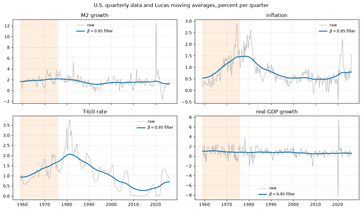
Money growth, inflation, and the interest rate rise together into the early 1980s and then fall together.
After 1984 that comovement is much harder to see, and the pandemic surge in M2 growth stands entirely apart from everything else.
139.5. Scatter plots#
Following the paper we plot second quarter observations of each year, which reduces the overlap between neighboring filtered values.
PERIODS = [('1959-1975', 1959, 1975), ('1960-1983', 1960, 1983),
           ('1984-2007', 1984, 2007), ('2008-present', 2008, 2100)]


def scatter_panel(yvar, title):
    q2 = filtered[filtered.index.quarter == 2]
    pad = 0.15 * (q2[['dm', yvar]].values.max() - q2[['dm', yvar]].values.min())
    lim = np.array([q2[['dm', yvar]].values.min() - pad,
                    q2[['dm', yvar]].values.max() + pad])
    fig, axes = plt.subplots(1, 4, figsize=(14, 3.8), sharex=True, sharey=True)
    for ax, (name, lo, hi) in zip(axes, PERIODS):
        sub = q2[(q2.index.year >= lo) & (q2.index.year <= hi)]
        x, y = sub['dm'].values, sub[yvar].values
        ax.scatter(x, y, s=26, color='C0')
        b = np.polyfit(x, y, 1)
        xx = np.linspace(x.min(), x.max(), 2)
        ax.plot(xx, np.polyval(b, xx), color='C3', lw=2,
                label=f'slope = {b[0]:.2f}')
        ax.plot(lim, lim, color='0.4', ls='--', lw=1, label='45 degrees')
        ax.set(xlim=lim, ylim=lim, title=name, xlabel='money growth')
        ax.legend(frameon=False, fontsize=8, loc='upper left')
    axes[0].set_ylabel(title)
    fig.suptitle(f'{title} against money growth, $\\beta = 0.95$ filtered')
    plt.tight_layout()
    plt.show()


scatter_panel('pi', 'inflation')
scatter_panel('R', 'interest rate')
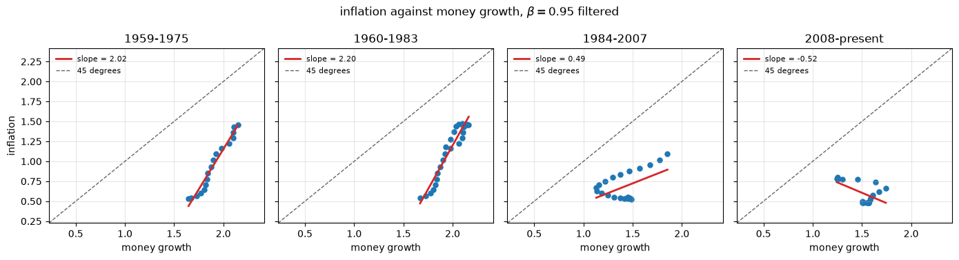
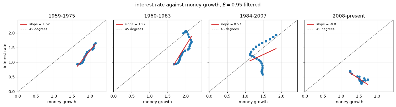
Lucas’s window and the pre-Volcker sample line up with the 45 degree line.
The great moderation and the period since 2008 do not.
139.6. Regressions on filtered data#
Table 1 of the paper reports these slopes for a grid of \(\beta\) values.
def filtered_slopes(betas=(0.95, 0.8, 0.5, 0.0)):
    rows = {}
    for beta in betas:
        f = pd.DataFrame({c: lucas_filter(data[c].values, beta) for c in VARS},
                         index=data.index)
        for name, lo, hi in PERIODS + [('full sample', 1900, 2100)]:
            m = ((f.index.year >= lo) & (f.index.year <= hi)
                 & (f.index.quarter == 2))
            x = f.loc[m, 'dm'].values
            rows.setdefault(name, {})[('pi on dm', beta)] = np.polyfit(x, f.loc[m, 'pi'], 1)[0]
            rows[name][('R on dm', beta)] = np.polyfit(x, f.loc[m, 'R'], 1)[0]
    tab = pd.DataFrame(rows).T
    order = [(v, b) for v in ['pi on dm', 'R on dm'] for b in betas]
    return tab.reindex(columns=order)


filtered_slopes().round(2)
| pi on dm | R on dm | |||||||
|---|---|---|---|---|---|---|---|---|
| 0.95 | 0.80 | 0.50 | 0.00 | 0.95 | 0.80 | 0.50 | 0.00 | |
| 1959-1975 | 2.02 | 1.06 | 0.24 | 0.01 | 1.52 | 0.54 | -0.02 | -0.12 |
| 1960-1983 | 2.20 | 1.14 | 0.23 | 0.04 | 1.97 | 0.94 | 0.15 | 0.05 |
| 1984-2007 | 0.49 | 0.02 | -0.04 | -0.03 | 0.57 | 0.23 | 0.21 | 0.08 |
| 2008-present | -0.52 | -0.09 | -0.05 | -0.08 | -0.81 | -0.34 | -0.15 | -0.06 |
| full sample | 0.85 | 0.38 | 0.10 | -0.04 | 0.90 | 0.29 | 0.04 | -0.03 |
Two patterns stand out.
The closer \(\beta\) is to one, the larger the slopes, exactly as in Lucas’s graphs and in the paper’s Table 1.
And the slopes fall steadily as we move through the sample, from above one in Lucas’s window to negative after 2008.
139.7. Estimates of \(h(0)\) from a VAR#
The filtered regressions are informal.
Equation (139.6) lets us compute \(h(0)\) properly from a fitted VAR.
We fit a VAR(2) in money growth, inflation, the interest rate, and output growth, put it in companion form, and read \(h(0)\) off the long-run multiplier matrix.
We use a diffuse prior so that we can report posterior bands, as the paper does in its Figure 5.
Draws whose companion matrix is explosive are discarded, since \(h(0)\) is not defined for them.
def bvar_h0(Y, p=2, n_draws=500, seed=0):
    """Posterior draws of h(0) from a VAR(p) under a diffuse prior."""
    rng = np.random.default_rng(seed)
    T, n = Y.shape
    X = np.column_stack([np.ones(T - p)] + [Y[p - l - 1:T - l - 1] for l in range(p)])
    Z, k = Y[p:], 1 + n * p
    XXi = np.linalg.inv(X.T @ X)
    B_hat = XXi @ X.T @ Z
    E = Z - X @ B_hat
    S, nu = E.T @ E, T - p - k
    L_x = np.linalg.cholesky(XXi)
    J = np.vstack([np.eye(n), np.zeros((n * (p - 1), n))])

    out = np.full((n_draws, 2), np.nan)
    for d in range(n_draws):
        Sigma = invwishart.rvs(df=nu, scale=S, random_state=rng)
        B = B_hat + L_x @ rng.standard_normal((k, n)) @ np.linalg.cholesky(Sigma).T
        A = np.zeros((n * p, n * p))
        A[:n] = np.hstack([B[1 + l * n:1 + (l + 1) * n].T for l in range(p)])
        if p > 1:
            A[n:, :n * (p - 1)] = np.eye(n * (p - 1))
        if np.max(abs(np.linalg.eigvals(A))) >= 1:
            continue
        G = np.linalg.solve(np.eye(n * p) - A, J)
        S0 = G @ Sigma @ G.T
        out[d] = [S0[1, 0] / S0[0, 0], S0[2, 0] / S0[0, 0]]
    return out
rows = []
for name, lo, hi in PERIODS + [('full sample', 1900, 2100)]:
    m = (data.index.year >= lo) & (data.index.year <= hi)
    o = bvar_h0(data.loc[m, VARS].values)
    qs = np.nanpercentile(o, [16, 50, 84], axis=0)
    rows.append(dict(period=name, T=int(m.sum()),
                     h_pi=qs[1, 0], h_pi_lo=qs[0, 0], h_pi_hi=qs[2, 0],
                     h_R=qs[1, 1], h_R_lo=qs[0, 1], h_R_hi=qs[2, 1]))
pd.DataFrame(rows).set_index('period').round(2)
| T | h_pi | h_pi_lo | h_pi_hi | h_R | h_R_lo | h_R_hi | |
|---|---|---|---|---|---|---|---|
| period | |||||||
| 1959-1975 | 67 | 1.26 | 0.22 | 2.36 | 0.61 | -0.04 | 1.31 |
| 1960-1983 | 96 | 0.74 | -0.31 | 1.90 | 0.61 | -0.63 | 1.91 |
| 1984-2007 | 96 | -0.07 | -0.30 | 0.14 | 0.27 | -0.29 | 0.81 |
| 2008-present | 74 | -0.17 | -0.64 | 0.37 | -0.59 | -1.16 | 0.25 |
| full sample | 269 | 0.73 | 0.45 | 1.08 | 0.99 | 0.44 | 1.61 |
The subperiods are chosen by hand, which is the objection that Boschen and Otrok [1994] raised against this style of evidence.
So we also run the VAR through rolling twenty year windows.
years = np.arange(data.index.year.min(), data.index.year.max() - 18)
mid, lo68, hi68 = {}, {}, {}
for y in years:
    m = (data.index.year >= y) & (data.index.year < y + 20)
    if m.sum() < 70:
        continue
    o = bvar_h0(data.loc[m, VARS].values, n_draws=300, seed=int(y))
    qs = np.nanpercentile(o, [16, 50, 84], axis=0)
    mid[y + 10], lo68[y + 10], hi68[y + 10] = qs[1], qs[0], qs[2]

mid = pd.DataFrame(mid).T
lo68, hi68 = pd.DataFrame(lo68).T, pd.DataFrame(hi68).T

fig, axes = plt.subplots(1, 2, figsize=(12, 4.2), sharex=True)
for j, (ax, ttl) in enumerate(zip(axes, [r'$h_{\pi,\Delta m}(0)$',
                                         r'$h_{R,\Delta m}(0)$'])):
    ax.plot(mid.index, mid[j], color='C3', lw=2, label='median')
    ax.fill_between(mid.index, lo68[j], hi68[j], color='C3', alpha=0.18,
                    label='68% band')
    ax.axhline(1, color='0.3', ls='--', lw=1, label='quantity theory')
    ax.axhline(0, color='0.7', lw=0.8)
    ax.set(title=ttl, xlabel='midpoint of 20 year window')
    ax.legend(frameon=False, fontsize=9)
fig.suptitle('Low-frequency slopes from rolling VARs')
plt.tight_layout()
plt.show()
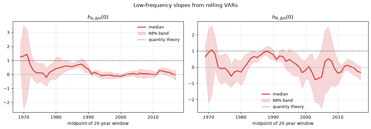
The two low-frequency slopes are high early in the sample, when Lucas wrote, and drift toward zero afterwards.
One is rarely inside the 68 percent band after the mid 1980s.
This is the instability that the rest of the lecture tries to explain.
139.8. A model for monetary policy analysis#
Section III of Sargent and Surico [2011] uses the log-linearized sticky price model of Ireland [2004], which has price indexation, habit formation, and a unit root technology shock.
The structure of the economy is
Here \(\pi_t\) is inflation, \(x_t\) the output gap, \(\Delta m_t\) nominal money growth, \(R_t\) the short rate, \(\tilde y_t\) detrended output, and \(z_t\) the growth rate of technology.
Equation (139.7) is a new Keynesian Phillips curve and (139.8) a new Keynesian IS curve.
Equation (139.9) is the money demand relation of McCallum and Nelson [1999] and Ireland [2003].
The discount factor is \(\theta\), \(\alpha_\pi\) is indexation to past inflation, \(\alpha_x\) is habit formation, \(\kappa\) is the slope of the Phillips curve, \(\sigma\) is the elasticity of intertemporal substitution, \(\tau\) is the Rotemberg [1982] price adjustment cost, \(\xi\) is the inverse Frisch elasticity, and \(1/\gamma\) is the interest semi-elasticity of money demand.
Four nonpolicy disturbances drive the economy: a markup shock \(e_t\), a demand shock \(a_t\), a money demand shock \(\chi_t\), and technology \(z_t\),
Monetary policy is either a money growth rule
or a Taylor rule
The observables are \([\Delta m_t, \pi_t, R_t, \Delta y_t]\).
139.9. Three things worth checking#
Before estimating anything it pays to look at what this parameterization can and cannot deliver.
139.9.1. \(\tau\) is not identified#
The price adjustment cost \(\tau\) enters the model in exactly one place, the term \(e_t/\tau\) in (139.7).
Since \(e_t\) is an AR(1) with a freely estimated innovation standard deviation \(\sigma_e\), the process \(e_t/\tau\) is an AR(1) with innovation standard deviation \(\sigma_e/\tau\).
So the likelihood depends on \((\tau, \sigma_e)\) only through the ratio \(\sigma_e/\tau\).
We verify this numerically below.
Table 2 of the paper nevertheless reports a posterior for \(\tau\) with mean 3.51 and a 5-95 interval of \([1.99, 4.99]\), against a prior with mean 4 and interval \([2.51, 5.77]\).
That posterior is not evidence about the Rotemberg adjustment cost.
Its leftward shift is what the prior on \(\sigma_e\) implies once the data pin down the ratio: the data want \(\sigma_e/\tau \approx 0.31\), while the inverse gamma prior on \(\sigma_e\) has mean \(0.3\) and pulls \(\sigma_e\) down, dragging \(\tau\) with it.
Because \(\tau\) contributes nothing, we fix it at its prior mean and estimate one fewer parameter.
Nothing in the fit, or in \(h(0)\), changes.
139.9.2. The first unit slope is an identity when money is exogenous#
Group the terms of the money demand equation (139.9) as
Everything other than \(\pi_t + z_t\) is a first difference.
The filter \(1 - e^{-i\omega}\) vanishes at \(\omega = 0\), so \(\Delta v_t\) contributes nothing to any spectral density or cross spectrum at frequency zero.
Therefore
This yields a proposition.
Proposition 139.1
Under the money growth rule (139.12) with \(\phi_\pi = \phi_x = 0\),
exactly, whatever the values of the other parameters.
Proof. With \(\phi_\pi = \phi_x = 0\) the rule reads \(\Delta m_t = \rho_m \Delta m_{t-1} + \varepsilon_{mt}\), so money growth is driven by \(\varepsilon_m\) alone.
From (139.14), \(\pi_t + z_t = \Delta m_t - \Delta v_t\), and \(\Delta v\) contributes nothing at frequency zero, so \(S_{z,\pi+z}(0) = S_{z,\Delta m}(0)\).
Technology is exogenous and orthogonal to \(\varepsilon_m\), so \(S_{z, \Delta m}(\omega) \equiv 0\).
Now apply (139.15).
This is worth thinking about.
Lucas’s first illustration prevails whenever money growth is econometrically exogenous, which is the case Whiteman [1984] assumed.
It is a property of the money demand specification, not of a deep monetary neutrality.
Departures from one arise only through \(S_{z,\pi+z}(0)\), and that term is nonzero only when the policy rule makes money growth respond to the endogenous variables, so that technology becomes correlated with money growth at frequency zero.
The second illustration has no such backing.
The same argument gives \(h_{R,\Delta m}(0) = S_{R,\pi+z}(0)/S_{\pi+z}(0)\), which equals one only if the low-frequency behavior of the ex ante real rate happens to cooperate.
So within this structural model, Lucas’s two illustrations are not on the same footing.
139.9.3. The reported posterior for \(\alpha_x\) stops at one half#
Table 2 reports a posterior for the habit parameter \(\alpha_x\) with mean 0.4775 and a 95th percentile of exactly 0.5000, under a beta prior on \([0,1]\).
An interval that ends on a round number is usually a constraint rather than a finding.
It is not a determinacy constraint: we check below that the model has a unique stable solution on both sides of \(\alpha_x = 0.5\).
We therefore let \(\alpha_x\) range over the whole unit interval.
139.10. Solving the model#
The model is a linear rational expectations system, which we solve with the method of Sims [2002].
Write it in the canonical form
where \(\varepsilon_t\) collects the structural shocks and \(\eta_t\) collects expectational errors, one for each variable whose expectation appears in the system.
The trick is to add \(\mathbb{E}_t \pi_{t+1}\) and \(\mathbb{E}_t x_{t+1}\) to the vector of variables, together with the identities
The solution algorithm takes a generalized Schur decomposition of the matrix pencil \((\Gamma_0, \Gamma_1)\), orders the stable generalized eigenvalues first, and then asks whether the expectational errors can be chosen to kill the explosive block.
If they can, a stable solution exists; if they can be chosen in only one way, it is unique.
SMALL = 1e-6


def gensys(g0, g1, psi, pi, div=1.01):
    """
    Solve  g0 @ y[t] = g1 @ y[t-1] + psi @ eps[t] + pi @ eta[t].

    Returns (G1, impact, eu) so that, when eu == (1, 1),

        y[t] = G1 @ y[t-1] + impact @ eps[t]

    is the unique stable solution.  eu[0] flags existence, eu[1] uniqueness.
    """
    n = g0.shape[0]
    S, T, alpha, beta, Q, Z = ordqz(g0, g1, output='complex',
                                    sort=lambda a, b: abs(b) < div * abs(a))
    nunstab = int(np.sum(abs(beta) >= div * abs(alpha)))
    ns = n - nunstab
    if np.any((abs(alpha) < SMALL) & (abs(beta) < SMALL)):
        return None, None, (-2, -2)

    q = Q.conj().T
    q1, q2 = q[:ns], q[ns:]

    def trimmed_svd(M):
        u, d, vh = svd(M)
        keep = d > SMALL
        r = len(d)
        return u[:, :r][:, keep], d[keep], vh.conj().T[:, :r][:, keep]

    u2, d2, v2 = trimmed_svd(q2 @ pi)        # can eta kill the explosive block?
    u1, d1, v1 = trimmed_svd(q1 @ pi)        # is the choice unique?

    exist = len(d2) >= nunstab
    if v1.shape[1] == 0:
        unique = True
    else:
        loose = v1 - v2 @ v2.conj().T @ v1
        unique = np.sum(svd(loose, compute_uv=False) > SMALL * n) == 0
    eu = (int(exist), int(unique))
    if not exist:
        return None, None, eu

    W = u2 @ np.diag(1 / d2) @ v2.conj().T @ v1 @ np.diag(d1) @ u1.conj().T
    tmat = np.hstack([np.eye(ns), -W.conj().T])
    G0 = np.vstack([tmat @ S,
                    np.hstack([np.zeros((nunstab, ns)), np.eye(nunstab)])])
    G0i = np.linalg.inv(G0)
    G1 = np.real(Z @ (G0i @ np.vstack([tmat @ T, np.zeros((nunstab, n))]))
                 @ Z.conj().T)
    impact = np.real(Z @ (G0i @ np.vstack([tmat @ q @ psi,
                                           np.zeros((nunstab, psi.shape[1]))])))
    return G1, impact, eu
Before trusting it, we check it against a model whose solution we can write down.
In the textbook three-equation new Keynesian model
with \(g_t\) an AR(1), the equilibrium is \(\pi_t = \pi_g g_t\) and \(x_t = x_g g_t\) where \((\pi_g, x_g)\) solves a two by two linear system, and the equilibrium is unique if and only if \(\phi_\pi > 1\).
def toy_nk(phi_pi, theta=0.99, kappa=0.1, sigma=1.0, rho=0.8):
    """y = [pi, x, R, g, E pi(+1), E x(+1)]."""
    g0, g1 = np.zeros((6, 6)), np.zeros((6, 6))
    psi, pie = np.zeros((6, 1)), np.zeros((6, 2))
    g0[0, 0], g0[0, 4], g0[0, 1] = 1, -theta, -kappa
    g0[1, 1], g0[1, 5], g0[1, 2], g0[1, 4], g0[1, 3] = 1, -1, sigma, -sigma, -1
    g0[2, 2], g0[2, 0] = 1, -phi_pi
    g0[3, 3], g1[3, 3], psi[3, 0] = 1, rho, 1
    g0[4, 0], g1[4, 4], pie[4, 0] = 1, 1, 1
    g0[5, 1], g1[5, 5], pie[5, 1] = 1, 1, 1
    return g0, g1, psi, pie


for phi in [0.5, 1.5, 3.0]:
    G1, impact, eu = gensys(*toy_nk(phi))
    msg = 'unique stable solution' if eu == (1, 1) else 'indeterminate'
    print(f'phi_pi = {phi}:  eu = {eu}  ({msg})')

theta, kappa, sigma, rho, phi = 0.99, 0.1, 1.0, 0.8, 1.5
M = np.array([[1 - theta * rho, -kappa], [sigma * (phi - rho), 1 - rho]])
exact = np.linalg.solve(M, np.array([0.0, 1.0]))
G1, impact, _ = gensys(*toy_nk(phi))
print(f'\nanalytic (pi_g, x_g) = {np.round(exact, 8)}')
print(f'gensys   (pi_g, x_g) = {np.round(impact[:2, 0], 8)}')
phi_pi = 0.5:  eu = (1, 0)  (indeterminate)
phi_pi = 1.5:  eu = (1, 1)  (unique stable solution)
phi_pi = 3.0:  eu = (1, 1)  (unique stable solution)

analytic (pi_g, x_g) = [0.89605735 1.86379928]
gensys   (pi_g, x_g) = [0.89605735 1.86379928]
The solver reproduces the analytic solution to machine precision and correctly refuses to deliver one when \(\phi_\pi < 1\).
139.11. The Sargent-Surico model in canonical form#
Now we write (139.7) through (139.13) in the form (139.16).
The vector of variables is
and the shocks are \(\varepsilon_t = [\varepsilon_{et}, \varepsilon_{at}, \varepsilon_{\chi t}, \varepsilon_{zt}, \varepsilon_{mt}]'\).
PI, X, DM, R, E, A_, CH, Z, EPI, EX = range(10)
NY = 10


def canonical(p, rule='money'):
    """Matrices g0, g1, psi, pi of equations (SS-NKPC) through (SS-Taylor)."""
    th, api, kap, tau = p['theta'], p['alpha_pi'], p['kappa'], p['tau']
    ax, sig, xi, gam = p['alpha_x'], p['sigma'], p['xi'], p['gamma']
    g0, g1 = np.zeros((NY, NY)), np.zeros((NY, NY))
    psi, pie = np.zeros((NY, 5)), np.zeros((NY, 2))

    # Phillips curve
    g0[0, PI], g0[0, EPI], g0[0, X], g0[0, E] = 1, -th * (1 - api), -kap, 1 / tau
    g1[0, PI] = th * api
    # IS curve
    g0[1, X], g0[1, EX], g0[1, R], g0[1, EPI] = 1, -(1 - ax), sig, -sig
    g0[1, A_] = -sig * (1 - xi) * (1 - p['rho_a'])
    g1[1, X] = ax
    # money demand
    g0[2, DM], g0[2, PI], g0[2, Z] = 1, -1, -1
    for col, coef in [(X, -1 / (sig * gam)), (R, 1 / gam),
                      (CH, -1 / gam), (A_, 1 / gam)]:
        g0[2, col], g1[2, col] = coef, coef
    # policy rule
    if rule == 'money':
        rm = p['rho_m']
        g0[3, DM] = 1
        g0[3, PI], g0[3, X] = -(1 - rm) * p['phi_pi'], -(1 - rm) * p['phi_x']
        g1[3, DM] = rm
    else:
        rr = p['rho_r']
        g0[3, R] = 1
        g0[3, PI], g0[3, X] = -(1 - rr) * p['psi_pi'], -(1 - rr) * p['psi_x']
        g1[3, R] = rr
    psi[3, 4] = 1
    # exogenous shocks
    for row, (v, rho, k) in enumerate([(E, p['rho_e'], 0), (A_, p['rho_a'], 1),
                                       (CH, p['rho_chi'], 2), (Z, 0.0, 3)], 4):
        g0[row, v], g1[row, v], psi[row, k] = 1, rho, 1
    # expectational identities
    g0[8, PI], g1[8, EPI], pie[8, 0] = 1, 1, 1
    g0[9, X], g1[9, EX], pie[9, 1] = 1, 1, 1
    return g0, g1, psi, pie
Output growth in (139.10) needs \(x_{t-1}\) and \(a_{t-1}\), so the state carries those two lags,
There is no measurement error, so \(D = 0\) and (139.6) applies directly.
The following issue arises here.
The div argument of gensys splits stable from explosive generalized eigenvalues, and it has to sit a little above one for the split to be numerically reliable.
So a solution that gensys reports as unique and stable can still have a root of the transition matrix at or just above one.
Both \(h(0)\) and the Kalman filter need covariance stationarity, so we test for it explicitly rather than trusting the flags.
def state_space(p, rule='money'):
    """
    Return A, B, C for S[t] = A S[t-1] + B eps[t] and Y[t] = C S[t],
    together with a status string that is 'ok' when the equilibrium is
    unique and covariance stationary.
    """
    G1, impact, eu = gensys(*canonical(p, rule))
    if eu[0] != 1:
        return None, None, None, 'no stable solution'
    if eu[1] != 1:
        return None, None, None, 'indeterminate'
    sd = np.diag([p['sig_e'], p['sig_a'], p['sig_chi'], p['sig_z'], p['sig_m']])
    n = NY + 2
    A, B = np.zeros((n, n)), np.zeros((n, 5))
    A[:NY, :NY] = G1
    A[NY, X], A[NY + 1, A_] = 1, 1
    B[:NY] = impact @ sd
    C = np.zeros((4, n))                              # [dm, pi, R, dy]
    C[0, DM], C[1, PI], C[2, R] = 1, 1, 1
    C[3, X], C[3, NY] = 1, -1
    C[3, A_], C[3, NY + 1] = p['xi'], -p['xi']
    C[3, Z] = 1
    if np.max(np.abs(np.linalg.eigvals(A))) > 1 - 1e-9:
        return None, None, None, 'unit or explosive root'
    return A, B, C, 'ok'


def h_zero(p, rule='money'):
    """(h_pi,dm(0), h_R,dm(0)) implied by the model at parameters p."""
    A, B, C, status = state_space(p, rule)
    if status != 'ok':
        return np.nan, np.nan
    return (h_zero_from_state_space(A, B, C, 1, 0),
            h_zero_from_state_space(A, B, C, 2, 0))
This test matters.
Without it, a point like \(\phi_\pi = 1\), \(\phi_x = 0\) returns \(h_{\pi,\Delta m}(0) = h_{R,\Delta m}(0) = 1.000\), an apparently perfect confirmation of both of Lucas’s illustrations.
The transition matrix there has a root of exactly one, the spectral density at frequency zero does not exist, and those two numbers come from inverting a matrix whose condition number is about \(10^{16}\).
That point sits in the upper right corner of the range that Figure 6 of the paper plots.
We show below that at the paper’s own Table 2 posterior means a whole strip of that range has no covariance stationary equilibrium.
We can now check our implementation against the paper.
At the posterior means of Table 2, Sargent and Surico [2011] report implied values \(h_{\pi,\Delta m}(0) = 1.0068\) and \(h_{R,\Delta m}(0) = 0.8163\).
PAPER = dict(theta=0.9901, alpha_pi=0.8815, kappa=0.0324, tau=3.5126,
             alpha_x=0.4775, sigma=0.0997, xi=3.0319, gamma=3.8128,
             phi_pi=0.2312, phi_x=-0.1971, rho_m=0.7428, rho_e=0.5645,
             rho_a=0.9241, rho_chi=0.5024, sig_e=1.0922, sig_a=0.7226,
             sig_chi=0.2388, sig_z=1.5845, sig_m=1.1457)

print('h at the posterior means of Table 2: %.4f, %.4f' % h_zero(PAPER))
print('reported in Table 2:                 1.0068, 0.8163')
h at the posterior means of Table 2: 1.0093, 0.8060
reported in Table 2:                 1.0068, 0.8163
Our independent implementation lands on the paper’s numbers.
That gives us confidence that we have read equations (139.7) through (139.12) the way their authors intended.
139.11.1. Checking the three claims#
Now we verify the three observations of the previous section.
print('scaling tau and sigma_e together leaves h(0) untouched:')
for f in [0.5, 1.0, 2.0, 8.0]:
    q = dict(PAPER, tau=PAPER['tau'] * f, sig_e=PAPER['sig_e'] * f)
    print(f'   tau, sigma_e scaled by {f:4.1f}:  h_pi = {h_zero(q)[0]:.10f}')

print('\nwith phi_pi = phi_x = 0, h_pi is exactly one for any other parameters:')
rng = np.random.default_rng(0)
for i in range(5):
    q = dict(PAPER, phi_pi=0.0, phi_x=0.0,
             kappa=rng.uniform(0.01, 0.3), alpha_pi=rng.uniform(0.1, 0.9),
             alpha_x=rng.uniform(0.1, 0.9), sigma=rng.uniform(0.05, 0.5),
             gamma=rng.uniform(1, 8), rho_m=rng.uniform(0, 0.95),
             sig_z=rng.uniform(0.2, 3.0), xi=rng.uniform(0.5, 5.0))
    print(f'   draw {i}:  h_pi = {h_zero(q)[0]:.12f}   h_R = {h_zero(q)[1]:.4f}')

print('\ndeterminacy on both sides of alpha_x = 0.5:')
for ax in [0.30, 0.45, 0.499, 0.501, 0.60, 0.80]:
    print(f'   alpha_x = {ax:5.3f}:  {state_space(dict(PAPER, alpha_x=ax))[3]}')
scaling tau and sigma_e together leaves h(0) untouched:
   tau, sigma_e scaled by  0.5:  h_pi = 1.0092936992
   tau, sigma_e scaled by  1.0:  h_pi = 1.0092936992
   tau, sigma_e scaled by  2.0:  h_pi = 1.0092936992
   tau, sigma_e scaled by  8.0:  h_pi = 1.0092936992

with phi_pi = phi_x = 0, h_pi is exactly one for any other parameters:
   draw 0:  h_pi = 1.000000000000   h_R = 0.4849
   draw 1:  h_pi = 1.000000000000   h_R = -0.0141
   draw 2:  h_pi = 1.000000000000   h_R = 0.2936
   draw 3:  h_pi = 1.000000000000   h_R = 0.7060
   draw 4:  h_pi = 1.000000000000   h_R = 0.7182

determinacy on both sides of alpha_x = 0.5:
   alpha_x = 0.300:  ok
   alpha_x = 0.450:  ok
   alpha_x = 0.499:  ok
   alpha_x = 0.501:  ok
   alpha_x = 0.600:  ok
   alpha_x = 0.800:  ok
All three claims hold.
The likelihood is invariant to scaling \((\tau, \sigma_e)\), the first unit slope is an identity under exogenous money growth, and the model is determinate on both sides of \(\alpha_x = 1/2\).
Notice also that \(h_{R,\Delta m}(0)\) moves all over the place across those same draws, which is the asymmetry between the two illustrations that Proposition 139.1 predicts.
Finally, here is the strip of the Figure 6 policy grid on which, at the paper’s own posterior means, no covariance stationary equilibrium exists.
for phi_x in [0.0, -0.25, -0.5]:
    bad = [round(g, 2) for g in np.linspace(-3, 1, 41)
           if state_space(dict(PAPER, phi_pi=g, phi_x=phi_x))[3] != 'ok']
    print(f'phi_x = {phi_x:5.2f}: no stationary equilibrium at phi_pi in '
          f'{bad if bad else "none of the grid"}')
phi_x =  0.00: no stationary equilibrium at phi_pi in [np.float64(-3.0), np.float64(-2.9), np.float64(-2.8), np.float64(-2.7), np.float64(-2.6), np.float64(-2.5), np.float64(-2.4), np.float64(-2.3), np.float64(-2.2), np.float64(-2.1), np.float64(-2.0), np.float64(-1.9), np.float64(-1.8), np.float64(-1.7), np.float64(-1.6), np.float64(1.0)]
phi_x = -0.25: no stationary equilibrium at phi_pi in none of the grid
phi_x = -0.50: no stationary equilibrium at phi_pi in none of the grid
The strip is far from the estimated policy rule, so the paper’s conclusions are not at stake.
But an \(h(0)\) reported over it would be a number computed from a spectral density that does not exist.
139.12. Bayesian estimation#
We estimate the money growth rule version on 1960:I-1983:IV, the paper’s sample.
The four observables are demeaned, since the model is written in deviations from a steady state.
mask = (data.index.year >= 1960) & (data.index.year <= 1983)
Y_est = data.loc[mask, VARS].values
Y_est = Y_est - Y_est.mean(0)
print(f'estimation sample: {mask.sum()} quarters, '
      f'{data.index[mask][0].date()} to {data.index[mask][-1].date()}')
estimation sample: 96 quarters, 1960-01-01 to 1983-10-01
139.12.1. The likelihood#
Given \((A, B, C)\) the likelihood follows from the Kalman filter.
We initialize the state at its unconditional mean and covariance, the latter solving the discrete Lyapunov equation \(P = A P A' + BB'\).
def loglik(p, Y, rule='money'):
    """Kalman filter log likelihood of Y (T x 4) at parameters p."""
    A, B, C, status = state_space(p, rule)
    if status != 'ok':
        return -np.inf
    Q = B @ B.T
    try:
        P = solve_discrete_lyapunov(A, Q)
    except Exception:
        return -np.inf
    s = np.zeros(A.shape[0])
    ll, const = 0.0, Y.shape[1] * np.log(2 * np.pi)
    for t in range(Y.shape[0]):
        s = A @ s
        P = A @ P @ A.T + Q
        v = Y[t] - C @ s                              # forecast error
        PCt = P @ C.T
        F = C @ PCt                                   # its covariance
        try:
            L = np.linalg.cholesky(F)
        except np.linalg.LinAlgError:
            return -np.inf
        u = np.linalg.solve(L, v)
        ll -= 0.5 * (const + 2 * np.sum(np.log(np.diag(L))) + u @ u)
        K = np.linalg.solve(F, PCt.T).T               # Kalman gain
        s, P = s + K @ v, P - K @ PCt.T
    return ll if np.isfinite(ll) else -np.inf
139.12.2. Priors#
We use the prior means and standard deviations of Table 2, matching moments to pick the parameters of each family.
def beta_prior(m, s):
    nu = m * (1 - m) / s ** 2 - 1
    return stats.beta(m * nu, (1 - m) * nu)


def gamma_prior(m, s):
    return stats.gamma(m ** 2 / s ** 2, scale=s ** 2 / m)


def invgamma_prior(m, s):
    a = m ** 2 / s ** 2 + 2
    return stats.invgamma(a, scale=m * (a - 1))


PRIOR, SUPPORT = {}, {}
for n, (m, s) in [('theta', (0.99, 0.005)), ('alpha_pi', (0.5, 0.2)),
                  ('alpha_x', (0.5, 0.2)), ('rho_m', (0.5, 0.05)),
                  ('rho_e', (0.5, 0.1)), ('rho_a', (0.5, 0.1)),
                  ('rho_chi', (0.5, 0.1))]:
    PRIOR[n], SUPPORT[n] = beta_prior(m, s), (1e-6, 1 - 1e-6)
for n, (m, s) in [('kappa', (0.3, 0.1)), ('sigma', (0.1, 0.05)),
                  ('xi', (2.0, 1.0)), ('gamma', (4.0, 1.0))]:
    PRIOR[n], SUPPORT[n] = gamma_prior(m, s), (1e-8, np.inf)
for n in ['phi_pi', 'phi_x']:
    PRIOR[n], SUPPORT[n] = stats.norm(0, 0.5), (-np.inf, np.inf)
for n in ['sig_e', 'sig_a', 'sig_chi', 'sig_z', 'sig_m']:
    PRIOR[n], SUPPORT[n] = invgamma_prior(0.3, 1.0), (1e-8, np.inf)

FREE = ['theta', 'alpha_pi', 'kappa', 'alpha_x', 'sigma', 'xi', 'gamma',
        'phi_pi', 'phi_x', 'rho_m', 'rho_e', 'rho_a', 'rho_chi',
        'sig_e', 'sig_a', 'sig_chi', 'sig_z', 'sig_m']
TAU = 4.0                       # not identified; fixed at its prior mean


def unpack(v):
    return dict({n: float(x) for n, x in zip(FREE, v)}, tau=TAU)


def log_post(v, Y):
    lp = 0.0
    for n, x in zip(FREE, v):
        lo, hi = SUPPORT[n]
        if not lo < x < hi:
            return -np.inf
        lp += PRIOR[n].logpdf(x)
    return lp + loglik(unpack(v), Y)
139.12.3. The posterior mode#
We start the search at the paper’s posterior means, use Powell’s derivative free method, and polish with a gradient method.
v_start = np.array([PAPER[n] for n in FREE])
neg_log_post = lambda v: -log_post(v, Y_est)

res = optimize.minimize(neg_log_post, v_start, method='Powell',
                        options=dict(maxiter=20000, maxfev=20000))
res = optimize.minimize(neg_log_post, res.x, method='L-BFGS-B',
                        bounds=[SUPPORT[n] for n in FREE])
v_mode = res.x
print(f'log posterior at the paper\'s means: {log_post(v_start, Y_est):10.3f}')
print(f'log posterior at the mode:          {-res.fun:10.3f}')
print('h(0) at the mode: %.4f, %.4f' % h_zero(unpack(v_mode)))
log posterior at the paper's means:   -531.052
log posterior at the mode:            -320.204
h(0) at the mode: 0.9765, 0.7694
Note
Starting the search at the paper’s estimates finds the mode nearest to them.
The Hamiltonian Monte Carlo section at the end of this lecture discovers that this is a local mode, and that the posterior has a second one with higher density.
139.12.4. Random walk Metropolis-Hastings#
The standard proposal covariance is the inverse Hessian of the negative log posterior at the mode, which we compute by finite differences.
def numerical_hessian(f, v, rel=1e-4):
    n = len(v)
    h = rel * np.maximum(np.abs(v), 1e-2)
    H = np.zeros((n, n))
    for i in range(n):
        for j in range(i, n):
            ei, ej = np.zeros(n), np.zeros(n)
            ei[i], ej[j] = h[i], h[j]
            H[i, j] = H[j, i] = (f(v + ei + ej) - f(v + ei - ej)
                                 - f(v - ei + ej) + f(v - ei - ej)) / (4 * h[i] * h[j])
    return H


H = numerical_hessian(neg_log_post, v_mode)
Sigma_prop = np.linalg.inv(H)
print('proposal covariance is positive definite:',
      np.all(np.linalg.eigvalsh(H) > 0))
proposal covariance is positive definite: True
def rwmh(Y, v0, Sigma, n_draws, c=0.45, seed=42):
    """Random walk Metropolis-Hastings in the natural parameter space."""
    rng = np.random.default_rng(seed)
    L = np.linalg.cholesky(Sigma)
    v, lp = v0.copy(), log_post(v0, Y)
    draws, n_acc = np.empty((n_draws, len(v))), 0
    for i in range(n_draws):
        cand = v + c * (L @ rng.standard_normal(len(v)))
        lp_cand = log_post(cand, Y)
        if np.log(rng.random()) < lp_cand - lp:
            v, lp, n_acc = cand, lp_cand, n_acc + 1
        draws[i] = v
    return draws, n_acc / n_draws
Draws that fall outside the support of a prior get \(-\infty\) and are rejected, so we can work in the natural parameter space and skip transformations.
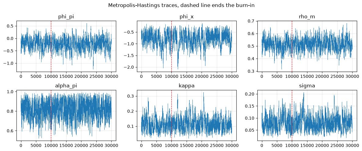
The chain below is short enough to run while you read; a serious application would use many more draws.
N_DRAWS, BURN = 30_000, 10_000

t0 = time.time()
draws, acc_rate = rwmh(Y_est, v_mode, Sigma_prop, N_DRAWS)
rwmh_seconds = time.time() - t0

kept = draws[BURN::5]
print(f'acceptance rate {acc_rate:.3f},  {len(kept)} retained draws, '
      f'{rwmh_seconds:.0f} seconds')
acceptance rate 0.283, 4000 retained draws, 275 seconds
fig, axes = plt.subplots(2, 3, figsize=(12, 5))
for ax, n in zip(axes.flat, ['phi_pi', 'phi_x', 'rho_m',
                             'alpha_pi', 'kappa', 'sigma']):
    j = FREE.index(n)
    ax.plot(draws[:, j], lw=0.4, color='C0')
    ax.axvline(BURN, color='C3', ls='--', lw=1)
    ax.set_title(n)
fig.suptitle('Metropolis-Hastings traces, dashed line ends the burn-in')
plt.tight_layout()
plt.show()
summary = pd.DataFrame({
    'prior mean': [PRIOR[n].mean() for n in FREE],
    'post. mean': kept.mean(0),
    '5th': np.percentile(kept, 5, axis=0),
    '95th': np.percentile(kept, 95, axis=0),
    'paper': [PAPER[n] for n in FREE]}, index=FREE)
summary.round(4)
| prior mean | post. mean | 5th | 95th | paper | |
|---|---|---|---|---|---|
| theta | 0.99 | 0.9887 | 0.9787 | 0.9960 | 0.9901 |
| alpha_pi | 0.50 | 0.8162 | 0.6641 | 0.9455 | 0.8815 |
| kappa | 0.30 | 0.1174 | 0.0581 | 0.1957 | 0.0324 |
| alpha_x | 0.50 | 0.3799 | 0.3026 | 0.4313 | 0.4775 |
| sigma | 0.10 | 0.0820 | 0.0396 | 0.1345 | 0.0997 |
| xi | 2.00 | 3.5793 | 2.1664 | 5.3518 | 3.0319 |
| gamma | 4.00 | 2.0430 | 1.5863 | 2.6046 | 3.8128 |
| phi_pi | 0.00 | -0.2361 | -0.6368 | 0.1261 | 0.2312 |
| phi_x | 0.00 | -0.7989 | -1.3512 | -0.3665 | -0.1971 |
| rho_m | 0.50 | 0.5162 | 0.4381 | 0.5949 | 0.7428 |
| rho_e | 0.50 | 0.2580 | 0.1561 | 0.3750 | 0.5645 |
| rho_a | 0.50 | 0.8499 | 0.7584 | 0.9133 | 0.9241 |
| rho_chi | 0.50 | 0.5169 | 0.3609 | 0.6777 | 0.5024 |
| sig_e | 0.30 | 1.1648 | 0.8815 | 1.4654 | 1.0922 |
| sig_a | 0.30 | 0.2468 | 0.1511 | 0.3717 | 0.7226 |
| sig_chi | 0.30 | 0.1408 | 0.0589 | 0.2533 | 0.2388 |
| sig_z | 0.30 | 0.7131 | 0.5513 | 0.9239 | 1.5845 |
| sig_m | 0.30 | 0.7143 | 0.6161 | 0.8311 | 1.1457 |
Our estimates are recognizably those of Table 2, with the differences one expects from a different interest rate series and different data vintages.
The Phillips curve is strongly backward looking and flat, the IS curve much less so.
Most important for what follows, the money growth rule responds weakly to inflation, with a posterior for \(\phi_\pi\) that straddles zero, and it carries substantial smoothing.
That is the paper’s central reading of the pre-1984 regime: the Federal Reserve put persistent, nearly exogenous, movement into money growth.
By Proposition 139.1 that is precisely the configuration in which Lucas’s first illustration holds, which is also why the paper’s own posterior for \(h_{\pi,\Delta m}(0)\) in Table 2 is so remarkably tight around one.
139.12.5. The posterior distribution of \(h(0)\)#
Every draw of the structural parameters implies a pair of low-frequency slopes.
h_draws = np.array([h_zero(unpack(v)) for v in kept])

fig, axes = plt.subplots(1, 2, figsize=(11, 3.8))
for ax, j, ttl in zip(axes, [0, 1],
                      [r'$h_{\pi,\Delta m}(0)$', r'$h_{R,\Delta m}(0)$']):
    ax.hist(h_draws[:, j], bins=60, color='C0', alpha=0.8, density=True)
    ax.axvline(1, color='0.3', ls='--', lw=1.5)
    ax.set_title(f'{ttl}   mean {h_draws[:, j].mean():.3f}, '
                 f'90% [{np.percentile(h_draws[:, j], 5):.3f}, '
                 f'{np.percentile(h_draws[:, j], 95):.3f}]')
fig.suptitle('Posterior of the low-frequency slopes implied by the model')
plt.tight_layout()
plt.show()
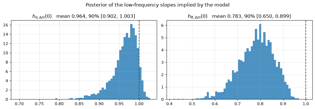
The estimated model reproduces Lucas’s two illustrations over a sample much like his.
Compare these with the VAR estimates for 1960-1983 that we computed earlier, and with the paper’s reported posterior means of 1.0068 and 0.8163.
139.13. How monetary policy moves the low-frequency slopes#
Now for the paper’s main experiment.
We lock every structural parameter at its posterior mean, vary only the two policy coefficients, and recompute \(h(0)\) at each point.
p_bar = unpack(kept.mean(0))


def h_grid(p, rule, k1, k2, g1_vals, g2_vals):
    H1 = np.full((len(g2_vals), len(g1_vals)), np.nan)
    H2 = np.full_like(H1, np.nan)
    for i, b in enumerate(g2_vals):
        for j, a in enumerate(g1_vals):
            H1[i, j], H2[i, j] = h_zero(dict(p, **{k1: a, k2: b}), rule)
    return H1, H2


phi_pi_grid = np.linspace(-3, 1, 49)
phi_x_grid = np.linspace(-1, 0, 25)
Hpi, HR = h_grid(p_bar, 'money', 'phi_pi', 'phi_x', phi_pi_grid, phi_x_grid)
def contour_panel(g1_vals, g2_vals, H1, H2, xlab, ylab, suptitle, scatter=None):
    fig, axes = plt.subplots(1, 2, figsize=(12, 4.4), sharey=True)
    for ax, Hm, ttl in zip(axes, [H1, H2],
                           [r'$h_{\pi,\Delta m}(0)$', r'$h_{R,\Delta m}(0)$']):
        cs = ax.contourf(g1_vals, g2_vals, Hm, levels=14, cmap='viridis')
        ax.contour(g1_vals, g2_vals, Hm, levels=[0.2, 1.0],
                   colors=['white', 'red'], linewidths=1.8)
        ax.contourf(g1_vals, g2_vals, np.isnan(Hm).astype(float),
                    levels=[0.5, 1.5], colors=['0.85'])
        if scatter is not None:
            ax.scatter(*scatter, s=1.5, color='k', alpha=0.25)
        fig.colorbar(cs, ax=ax)
        ax.set(title=ttl, xlabel=xlab)
    axes[0].set_ylabel(ylab)
    fig.suptitle(suptitle)
    plt.tight_layout()
    plt.show()


contour_panel(phi_pi_grid, phi_x_grid, Hpi, HR, r'$\phi_\pi$', r'$\phi_x$',
              'Low-frequency slopes under the money growth rule\n'
              '(white contour: 0.2, red contour: 1.0, dots: posterior draws)',
              scatter=(kept[:, FREE.index('phi_pi')],
                       kept[:, FREE.index('phi_x')]))
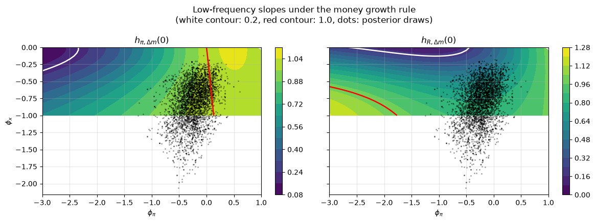
Three things come through, and they are the paper’s three findings.
The low-frequency slopes are not policy invariant: moving \((\phi_\pi, \phi_x)\) alone sweeps \(h_{\pi,\Delta m}(0)\) across most of the range that the rolling VARs displayed.
The cloud of posterior draws sits in the region where both slopes are near one, which is where the 1960-1983 data put us.
And a much more aggressive anti-inflation stance, meaning a large negative \(\phi_\pi\) so that money growth is cut hard when inflation rises, moves both slopes far below one, with the smallest values in the corner where \(\phi_x\) is also near zero.
The red contour marks \(h(0) = 1\) and, as Proposition 139.1 requires, it passes exactly through \(\phi_\pi = \phi_x = 0\).
Any gray region would be one with no unique covariance stationary equilibrium, where \(h(0)\) does not exist.
Here is where the slopes bottom out, a slice through the grid at the posterior mean of \(\phi_x\), and the fraction of the grid the stationarity test removes.
print(f'no stationary equilibrium at {np.isnan(Hpi).mean():.0%} of grid points')
for name, Hm in [('h_pi', Hpi), ('h_R', HR)]:
    i, j = np.unravel_index(np.nanargmin(Hm), Hm.shape)
    print(f'   smallest {name:5s} = {Hm[i, j]:6.3f} at '
          f'phi_pi = {phi_pi_grid[j]:5.2f}, phi_x = {phi_x_grid[i]:5.2f}')

row = np.argmin(np.abs(phi_x_grid - p_bar['phi_x']))
print(f'\nslice at phi_x = {phi_x_grid[row]:.3f}')
for j in range(0, len(phi_pi_grid), 6):
    print(f'   phi_pi = {phi_pi_grid[j]:6.2f}:  '
          f'h_pi = {Hpi[row, j]:7.3f},  h_R = {HR[row, j]:7.3f}')
no stationary equilibrium at 0% of grid points
   smallest h_pi  =  0.097 at phi_pi = -3.00, phi_x =  0.00
   smallest h_R   =  0.059 at phi_pi = -1.25, phi_x =  0.00

slice at phi_x = -0.792
   phi_pi =  -3.00:  h_pi =   0.463,  h_R =   1.137
   phi_pi =  -2.50:  h_pi =   0.550,  h_R =   1.056
   phi_pi =  -2.00:  h_pi =   0.646,  h_R =   0.972
   phi_pi =  -1.50:  h_pi =   0.748,  h_R =   0.892
   phi_pi =  -1.00:  h_pi =   0.847,  h_R =   0.828
   phi_pi =  -0.50:  h_pi =   0.933,  h_R =   0.796
   phi_pi =   0.00:  h_pi =   0.992,  h_R =   0.808
   phi_pi =   0.50:  h_pi =   1.017,  h_R =   0.870
   phi_pi =   1.00:  h_pi =   1.005,  h_R =   0.980
139.13.1. The same exercise with a Taylor rule#
The paper repeats the experiment with the interest rate rule (139.13).
We keep the smoothing coefficient and the policy shock standard deviation at their money rule estimates and vary \((\psi_\pi, \psi_x)\).
Where the Taylor rule leaves the equilibrium indeterminate we simply record it, shading those regions in gray; the paper instead selects the orthogonality solution of Lubik and Schorfheide [2004].
p_taylor = dict(p_bar, rho_r=p_bar['rho_m'], psi_pi=1.5, psi_x=0.5)
psi_pi_grid = np.linspace(0, 3, 37)
psi_x_grid = np.linspace(0, 1, 21)
Tpi, TR = h_grid(p_taylor, 'taylor', 'psi_pi', 'psi_x',
                 psi_pi_grid, psi_x_grid)

print(f'indeterminate or nonexistent at {np.isnan(Tpi).mean():.0%} of grid points')
print(f'h_pi ranges over [{np.nanmin(Tpi):.2f}, {np.nanmax(Tpi):.2f}]')
print(f'h_R  ranges over [{np.nanmin(TR):.2f}, {np.nanmax(TR):.2f}]')

contour_panel(psi_pi_grid, psi_x_grid, Tpi, TR, r'$\psi_\pi$', r'$\psi_x$',
              'Low-frequency slopes under a Taylor rule\n'
              '(gray: no unique stable equilibrium)')
indeterminate or nonexistent at 33% of grid points
h_pi ranges over [0.70, 1.00]
h_R  ranges over [0.89, 1.87]
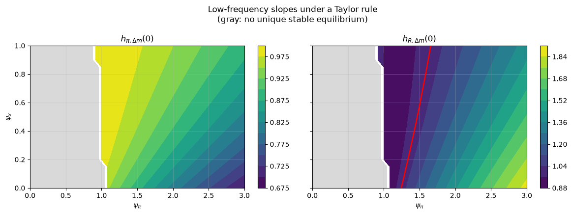
The dependence on policy survives, but it is much weaker.
Over the determinate region the Taylor rule cannot drive either slope anywhere near zero.
This is the paper’s finding that the interest rate rule is “less able to replicate the estimates.”
The decomposition (139.15) supplies a reason.
Driving \(h_{\pi,\Delta m}(0)\) toward zero requires making the ratio \(S_{z,\pi+z}(0)/S_{\pi+z}(0)\) close to one, which in practice means squeezing the zero-frequency power of inflation until \(\pi_t + z_t\) is dominated by technology.
A money growth rule with a large negative \(\phi_\pi\) does exactly that, because the central bank is choosing the left side of (139.14) directly.
A Taylor rule instead sets the interest rate and lets money growth be whatever money demand implies, so it never gets much purchase on low-frequency inflation relative to money growth, and \(h_{\pi,\Delta m}(0)\) stays near one.
139.14. Estimating with Hamiltonian Monte Carlo#
The random walk sampler that produced our posterior is the traditional workhorse of DSGE estimation.
It is also wasteful, and we can measure how wasteful.
This section takes the Sargent-Surico model as a guinea pig for a modern alternative.
139.14.1. What the random walk delivers#
A correlated chain of length \(N\) is worth fewer than \(N\) independent draws, and the effective sample size says how many.
import arviz as az

rwmh_idata = az.from_dict(
    {'posterior': {n: kept[:, j][None, :] for j, n in enumerate(FREE)}})
rwmh_summary = az.summary(rwmh_idata, var_names=FREE)
print(rwmh_summary[['mean', 'sd', 'ess_bulk']].to_string())
print(f'\n{len(kept)} retained draws out of {N_DRAWS}, in {rwmh_seconds:.0f} seconds')
print(f'smallest effective sample size = {rwmh_summary["ess_bulk"].min():.0f}')
            mean      sd ess_bulk
theta     0.9887  0.0053      197
alpha_pi   0.816   0.085      415
kappa      0.117   0.045      195
alpha_x     0.38   0.039      112
sigma      0.082   0.029      165
xi           3.6       1      111
gamma       2.04     0.3      125
phi_pi     -0.24    0.24      220
phi_x       -0.8    0.31       91
rho_m      0.516   0.047      221
rho_e      0.258   0.065      328
rho_a       0.85   0.047       53
rho_chi     0.52   0.096      307
sig_e       1.16    0.17      279
sig_a       0.25   0.068       93
sig_chi    0.141   0.061      200
sig_z       0.71    0.12       96
sig_m       0.71   0.065      149

4000 retained draws out of 30000, in 275 seconds
smallest effective sample size = 53
Tens of thousands of iterations buy us on the order of a hundred independent draws for the worst-mixing parameter.
The reason is visible in the proposal.
A random walk perturbs all eighteen parameters in a direction that knows nothing about the local shape of the posterior, so the step size has to respect the most tightly constrained direction while the loosest direction is explored at that same crawl.
Our posterior is badly scaled.
w = np.linalg.eigvalsh(H)
print(f'condition number of the posterior Hessian     {w.max() / w.min():10.3g}')
print(f'ratio of longest to shortest posterior scale  {np.sqrt(w.max() / w.min()):10.0f}')
condition number of the posterior Hessian        4.1e+04
ratio of longest to shortest posterior scale         202
139.14.2. Why Hamiltonian methods are awkward for DSGE models#
Hamiltonian Monte Carlo [Duane et al., 1987, Neal, 2011] treats the parameter vector as the position of a particle, gives it a random momentum, and simulates Hamiltonian dynamics in which the negative log posterior plays the role of potential energy.
Trajectories follow the contours of the distribution instead of blundering across them, so a proposal can travel a long way and still be accepted.
The No-U-Turn sampler [Hoffman and Gelman, 2014] removes the need to tune the trajectory length by extending each trajectory until it starts to double back on itself.
Betancourt [2017] gives a conceptual introduction.
The price of admission is the gradient \(\nabla_\theta \log p(\theta \mid Y)\).
That is where DSGE models become awkward.
Our likelihood runs through gensys, whose first act is an ordered generalized
Schur decomposition: it computes generalized eigenvalues, sorts them by modulus,
and reorders the decomposition to match.
Sorting is a discrete operation, and no automatic differentiation library propagates derivatives through it.
This, rather than any statistical objection, is the reason Hamiltonian methods remain uncommon in DSGE estimation.
139.14.3. A differentiable solver#
The obstacle is the algorithm, not the model, so we change algorithms.
Write the equilibrium conditions as
where
and \(u_t = \varepsilon_{mt}\) carries the money rule shock.
The auxiliary expectation variables that gensys needs are not required here.
Conjecture a solution
Then \(\mathbb{E}_t y_{t+1} = G y_t\), and (139.17) becomes
Solving for \(y_t\) and matching coefficients with (139.18) gives a fixed point in \(G\) alone,
Iterating (139.19) from \(G = 0\) involves nothing but matrix products and linear solves, every one of them differentiable.
import jax
import jax.numpy as jnp
import numpyro
import numpyro.distributions as dist
from jax import lax
from numpyro.infer import MCMC, NUTS

jax.config.update('jax_enable_x64', True)
jax.config.update('jax_platform_name', 'cpu')

U, NJ = 8, 9          # y = [pi, x, dm, R, e, a, chi, z, u]


def structural(p):
    """Return F_A, F_B, F_C, F_E of equation (SS-structural)."""
    th, api, kap = p['theta'], p['alpha_pi'], p['kappa']
    ax, sig, xi, gam = p['alpha_x'], p['sigma'], p['xi'], p['gamma']
    rm, ra = p['rho_m'], p['rho_a']
    FA = jnp.zeros((NJ, NJ)); FB = jnp.zeros((NJ, NJ))
    FC = jnp.zeros((NJ, NJ)); FE = jnp.zeros((NJ, 5))

    FA = FA.at[0, PI].set(-th * (1 - api))                        # Phillips curve
    FB = FB.at[0, PI].set(1).at[0, X].set(-kap).at[0, E].set(1 / TAU)
    FC = FC.at[0, PI].set(-th * api)

    FA = FA.at[1, X].set(-(1 - ax)).at[1, PI].set(-sig)           # IS curve
    FB = (FB.at[1, X].set(1).at[1, R].set(sig)
            .at[1, A_].set(-sig * (1 - xi) * (1 - ra)))
    FC = FC.at[1, X].set(-ax)

    FB = FB.at[2, DM].set(1).at[2, PI].set(-1).at[2, Z].set(-1)   # money demand
    FB = (FB.at[2, X].set(-1 / (sig * gam)).at[2, R].set(1 / gam)
            .at[2, CH].set(-1 / gam).at[2, A_].set(1 / gam))
    FC = (FC.at[2, X].set(1 / (sig * gam)).at[2, R].set(-1 / gam)
            .at[2, CH].set(1 / gam).at[2, A_].set(-1 / gam))

    FB = (FB.at[3, DM].set(1).at[3, U].set(-1)                    # policy rule
            .at[3, PI].set(-(1 - rm) * p['phi_pi'])
            .at[3, X].set(-(1 - rm) * p['phi_x']))
    FC = FC.at[3, DM].set(-rm)

    for row, (v, rho, k) in enumerate([(E, p['rho_e'], 0), (A_, ra, 1),
                                       (CH, p['rho_chi'], 2), (Z, 0.0, 3)], 4):
        FB = FB.at[row, v].set(1)
        FC = FC.at[row, v].set(-rho)
        FE = FE.at[row, k].set(-1)
    FB = FB.at[8, U].set(1)
    FE = FE.at[8, 4].set(-1)
    return FA, FB, FC, FE


def solve_fixed_point(p, n_iter=60):
    """Iterate (SS-fixedpoint) to convergence; differentiable throughout."""
    FA, FB, FC, FE = structural(p)

    def step(G, _):
        return -jnp.linalg.solve(FA @ G + FB, FC), None

    G, _ = lax.scan(step, jnp.zeros((NJ, NJ)), None, length=n_iter)
    return G, -jnp.linalg.solve(FA @ G + FB, FE)
Before trusting it we check it against gensys at the paper’s posterior means.
The two algorithms share no code, so agreement to machine precision is a real test.
p_check = {n: float(PAPER[n]) for n in FREE}
G_fp, Theta_fp = solve_fixed_point(p_check)

A_gen, B_gen, C_gen, _ = state_space(dict(p_check, tau=TAU))
idx = [PI, X, DM, R, E, A_, CH, Z]
sd_check = np.array([p_check[n] for n in
                     ['sig_e', 'sig_a', 'sig_chi', 'sig_z', 'sig_m']])

print('fixed point versus gensys')
print(f'   transition matrix  max abs difference  '
      f'{np.abs(np.asarray(G_fp)[np.ix_(idx, idx)] - A_gen[:10, :10][np.ix_(idx, idx)]).max():.2e}')
print(f'   shock loadings     max abs difference  '
      f'{np.abs(np.asarray(Theta_fp * sd_check)[idx] - B_gen[:10][idx]).max():.2e}')
fixed point versus gensys
   transition matrix  max abs difference  1.20e-14
   shock loadings     max abs difference  3.50e-15
Note
The fixed point converges to the stable solution when there is one, but unlike
gensys it returns no existence and uniqueness flags.
We therefore keep gensys for the determinacy map of the previous section and use
the fixed point only where we need derivatives.
139.14.4. The likelihood in JAX#
The Kalman filter carries over unchanged, written with lax.scan so that it too
can be differentiated.
The only substantive change is the initial covariance: instead of calling a Lyapunov solver we use \(\operatorname{vec}(P) = (I - A \otimes A)^{-1}\operatorname{vec}(Q)\), which is one linear solve.
def state_space_jax(p):
    G, Theta = solve_fixed_point(p)
    sd = jnp.array([p['sig_e'], p['sig_a'], p['sig_chi'], p['sig_z'], p['sig_m']])
    n = NJ + 2                                   # append x(-1) and a(-1)
    A = jnp.zeros((n, n)).at[:NJ, :NJ].set(G)
    A = A.at[NJ, X].set(1).at[NJ + 1, A_].set(1)
    B = jnp.zeros((n, 5)).at[:NJ].set(Theta * sd)
    C = jnp.zeros((4, n))
    C = C.at[0, DM].set(1).at[1, PI].set(1).at[2, R].set(1)
    C = C.at[3, X].set(1).at[3, NJ].set(-1)
    C = C.at[3, A_].set(p['xi']).at[3, NJ + 1].set(-p['xi'])
    C = C.at[3, Z].set(1)
    return A, B, C


def loglik_jax(p, Y):
    A, B, C = state_space_jax(p)
    n = A.shape[0]
    Q = B @ B.T
    P0 = jnp.linalg.solve(jnp.eye(n * n) - jnp.kron(A, A),
                          Q.reshape(-1)).reshape(n, n)
    const = Y.shape[1] * jnp.log(2 * jnp.pi)

    def step(carry, y):
        s, P = carry
        s, P = A @ s, A @ P @ A.T + Q
        v = y - C @ s
        PCt = P @ C.T
        F = C @ PCt
        L = jnp.linalg.cholesky(F)
        u = jax.scipy.linalg.solve_triangular(L, v, lower=True)
        ll = -0.5 * (const + 2 * jnp.sum(jnp.log(jnp.diag(L))) + u @ u)
        K = jnp.linalg.solve(F, PCt.T).T
        return (s + K @ v, P - K @ PCt.T), ll

    _, lls = lax.scan(step, (jnp.zeros(n), P0), Y)
    return jnp.sum(lls)
Two checks: the new likelihood must agree with the one we used for the random walk, and its gradient must agree with finite differences.
Y_jax = jnp.asarray(Y_est)
print(f'log likelihood, JAX    {float(loglik_jax(p_check, Y_jax)):.8f}')
print(f'log likelihood, NumPy  {loglik(dict(p_check, tau=TAU), Y_est):.8f}')

grad_ll = jax.jit(jax.grad(lambda q: loglik_jax(q, Y_jax)))
g = grad_ll(p_check)

print('\n                  autodiff    finite difference')
for n in ['phi_pi', 'kappa', 'rho_m', 'sig_z']:
    step_n = 1e-5
    up = dict(p_check); up[n] = p_check[n] + step_n
    dn = dict(p_check); dn[n] = p_check[n] - step_n
    fd = (loglik_jax(up, Y_jax) - loglik_jax(dn, Y_jax)) / (2 * step_n)
    print(f'   {n:8s} {float(g[n]):12.5f} {float(fd):17.5f}')
log likelihood, JAX    -493.21564637
log likelihood, NumPy  -493.21564637

                  autodiff    finite difference
   phi_pi       -1.00005          -1.00005
   kappa        -0.68555          -0.68555
   rho_m         1.92667           1.92667
   sig_z       -56.71510         -56.71510
t0 = time.time()
for _ in range(20):
    gg = grad_ll(p_check)
jax.block_until_ready(gg)
grad_ms = 1000 * (time.time() - t0) / 20

t0 = time.time()
for _ in range(20):
    loglik(dict(p_check, tau=TAU), Y_est)
loglik_ms = 1000 * (time.time() - t0) / 20

print(f'one NumPy log likelihood        {loglik_ms:6.2f} ms')
print(f'one JAX gradient (18 partials)  {grad_ms:6.2f} ms')
one NumPy log likelihood          7.80 ms
one JAX gradient (18 partials)    5.34 ms
A full gradient costs about what a single likelihood evaluation costs, which is the whole point of reverse-mode differentiation.
A finite-difference gradient would need at least nineteen likelihood evaluations.
139.14.5. Sampling with NUTS#
We hand the same priors to NumPyro [Phan et al., 2019], which supplies NUTS and handles the transformations to unconstrained space that Hamiltonian dynamics require.
def beta_np(m, s):
    nu = m * (1 - m) / s ** 2 - 1
    return dist.Beta(m * nu, (1 - m) * nu)


def gamma_np(m, s):
    return dist.Gamma(m ** 2 / s ** 2, m / s ** 2)


def invgamma_np(m, s):
    a = m ** 2 / s ** 2 + 2
    return dist.InverseGamma(a, m * (a - 1))


PRIORS_NP = {
    'theta': beta_np(0.99, 0.005), 'alpha_pi': beta_np(0.5, 0.2),
    'alpha_x': beta_np(0.5, 0.2), 'rho_m': beta_np(0.5, 0.05),
    'rho_e': beta_np(0.5, 0.1), 'rho_a': beta_np(0.5, 0.1),
    'rho_chi': beta_np(0.5, 0.1),
    'kappa': gamma_np(0.3, 0.1), 'sigma': gamma_np(0.1, 0.05),
    'xi': gamma_np(2.0, 1.0), 'gamma': gamma_np(4.0, 1.0),
    'phi_pi': dist.Normal(0, 0.5), 'phi_x': dist.Normal(0, 0.5),
    'sig_e': invgamma_np(0.3, 1.0), 'sig_a': invgamma_np(0.3, 1.0),
    'sig_chi': invgamma_np(0.3, 1.0), 'sig_z': invgamma_np(0.3, 1.0),
    'sig_m': invgamma_np(0.3, 1.0)}


def ss_model(Y):
    p = {n: numpyro.sample(n, PRIORS_NP[n]) for n in FREE}
    numpyro.factor('loglik', loglik_jax(p, Y))
Three settings matter.
We ask for a dense mass matrix, because the condition number reported above says the posterior has correlations that a diagonal preconditioner cannot absorb.
We cap the trajectory length, since without a cap NUTS spends most of its time on very long trajectories in the flattest directions.
And we run four chains rather than one, all started from the posterior mode.
That last choice is the one that earns its keep.
kernel = NUTS(ss_model, target_accept_prob=0.8, dense_mass=True,
              max_tree_depth=8,
              init_strategy=numpyro.infer.init_to_value(
                  values={n: float(v) for n, v in zip(FREE, v_mode)}))
mcmc = MCMC(kernel, num_warmup=400, num_samples=400, num_chains=4,
            chain_method='sequential', progress_bar=False)

t0 = time.time()
mcmc.run(jax.random.PRNGKey(1), Y_jax, extra_fields=('num_steps', 'diverging'))
jax.block_until_ready(mcmc.get_samples())
nuts_seconds = time.time() - t0

extra = mcmc.get_extra_fields()
print(f'{nuts_seconds:.0f} seconds for 4 chains of 400 draws')
print(f'mean leapfrog steps per iteration  '
      f'{np.asarray(extra["num_steps"]).mean():.0f}')
print(f'divergences                        '
      f'{int(np.asarray(extra["diverging"]).sum())}')
345 seconds for 4 chains of 400 draws
mean leapfrog steps per iteration  12
divergences                        0
nuts_idata = az.from_numpyro(mcmc)
nuts_summary = az.summary(nuts_idata, var_names=FREE,
                          ci_kind='hdi', ci_prob=0.94)
nuts_kept = np.column_stack([np.asarray(mcmc.get_samples()[n]) for n in FREE])
nuts_summary[['mean', 'sd', 'hdi94_lb', 'hdi94_ub', 'ess_bulk', 'r_hat']]
| mean | sd | hdi94_lb | hdi94_ub | ess_bulk | r_hat | |
|---|---|---|---|---|---|---|
| theta | 0.9891 | 0.0054 | 0.98 | 1 | 1853 | 1.00 |
| alpha_pi | 0.5 | 0.341 | 0.045 | 0.93 | 6 | 1.74 |
| kappa | 0.109 | 0.044 | 0.036 | 0.19 | 1539 | 1.01 |
| alpha_x | 0.388 | 0.04 | 0.31 | 0.46 | 744 | 1.01 |
| sigma | 0.086 | 0.03 | 0.034 | 0.14 | 1381 | 1.01 |
| xi | 3.54 | 1.02 | 1.8 | 5.5 | 1955 | 1.00 |
| gamma | 1.9 | 0.28 | 1.4 | 2.4 | 21 | 1.13 |
| phi_pi | -0.4 | 0.26 | -0.89 | 0.07 | 20 | 1.14 |
| phi_x | -0.88 | 0.3 | -1.5 | -0.38 | 53 | 1.06 |
| rho_m | 0.515 | 0.046 | 0.42 | 0.6 | 1356 | 1.00 |
| rho_e | 0.5 | 0.285 | 0.17 | 0.89 | 6 | 1.73 |
| rho_a | 0.84 | 0.049 | 0.74 | 0.92 | 664 | 1.02 |
| rho_chi | 0.509 | 0.098 | 0.34 | 0.69 | 1865 | 1.01 |
| sig_e | 0.8 | 0.402 | 0.26 | 1.3 | 6 | 1.73 |
| sig_a | 0.248 | 0.074 | 0.13 | 0.38 | 1823 | 1.01 |
| sig_chi | 0.149 | 0.077 | 0.038 | 0.29 | 1706 | 1.00 |
| sig_z | 0.73 | 0.11 | 0.53 | 0.94 | 246 | 1.03 |
| sig_m | 0.723 | 0.068 | 0.6 | 0.85 | 908 | 1.02 |
139.14.6. A warning sign in the diagnostics#
Most parameters look excellent, with \(\hat R\) at one and effective sample sizes in the hundreds or thousands.
A few do not, and it is worth asking which.
worst = nuts_summary['ess_bulk'].nsmallest(3).index.tolist()
print('weakest mixing:')
print(nuts_summary.loc[worst, ['mean', 'sd', 'ess_bulk', 'r_hat']])

by_chain = mcmc.get_samples(group_by_chain=True)
print('\nper-chain posterior means')
print(f'{"":10s}' + ''.join(f'{"chain " + str(c):>10s}' for c in range(4)))
for n in worst:
    v = np.asarray(by_chain[n])
    print(f'{n:10s}' + ''.join(f'{v[c].mean():10.4f}' for c in range(4)))
weakest mixing:
         mean     sd ess_bulk r_hat
alpha_pi  0.5  0.341        6  1.74
rho_e     0.5  0.285        6  1.73
sig_e     0.8  0.402        6  1.73

per-chain posterior means
             chain 0   chain 1   chain 2   chain 3
alpha_pi      0.1419    0.1489    0.8085    0.8041
rho_e         0.8193    0.8171    0.2574    0.2618
sig_e         0.3776    0.3770    1.1375    1.1328
The chains started from a common point, so any disagreement between them means some of them have wandered somewhere the others have not.
The identity of the badly behaved parameters is a clue.
Inflation in the data is persistent, and equation (139.7) offers two ways to deliver that persistence.
Intrinsic persistence comes from indexation to past inflation, a large \(\alpha_\pi\), with the markup shock left transitory.
Inherited persistence comes from a persistent markup shock, a large \(\rho_e\), with little indexation.
The parameters that mix worst are exactly the ones that distinguish these two stories.
That is a reason to suspect the posterior has more than one mode, and it tells us where to look for the second one.
139.14.7. Two modes#
Sampler diagnostics are a noisy instrument, so we settle the question with the optimizer instead.
Our mode search in the estimation section started from the paper’s posterior means and climbed to a high-indexation mode.
We now start the same optimizer from the opposite corner.
v_start_a = v_mode.copy()
for n, val in [('alpha_pi', 0.12), ('rho_e', 0.84), ('sig_e', 0.35)]:
    v_start_a[FREE.index(n)] = val

res_a = optimize.minimize(neg_log_post, v_start_a, method='Powell',
                          options=dict(maxiter=20000, maxfev=20000))
res_a = optimize.minimize(neg_log_post, res_a.x, method='L-BFGS-B',
                          bounds=[SUPPORT[n] for n in FREE])
v_mode_a = res_a.x

print(f'log posterior, low-indexation mode   {-res_a.fun:10.3f}')
print(f'log posterior, high-indexation mode  {log_post(v_mode, Y_est):10.3f}')
print('\n                low-index   high-index      paper')
for n in ['alpha_pi', 'rho_e', 'sig_e', 'kappa', 'phi_pi', 'phi_x']:
    i = FREE.index(n)
    print(f'   {n:9s}{v_mode_a[i]:10.4f}{v_mode[i]:13.4f}{PAPER[n]:11.4f}')
log posterior, low-indexation mode     -318.746
log posterior, high-indexation mode    -320.204

                low-index   high-index      paper
   alpha_pi     0.1096       0.8296     0.8815
   rho_e        0.8376       0.2359     0.5645
   sig_e        0.3288       1.1516     1.0922
   kappa        0.0817       0.0967     0.0324
   phi_pi      -0.4359      -0.1957     0.2312
   phi_x       -0.7975      -0.5739    -0.1971
There are two distinct modes, and the low-indexation one has the higher posterior density.
The mode we found earlier, the one nearest the paper’s published estimates and the one our random walk explored for thirty thousand draws, is a local mode.
The pooled NUTS draws show the same thing from the sampling side.
fig, axes = plt.subplots(1, 3, figsize=(13, 3.8))
for ax, n, ttl in zip(axes, ['alpha_pi', 'rho_e', 'sig_e'],
                      [r'$\alpha_\pi$: indexation',
                       r'$\rho_e$: markup persistence',
                       r'$\sigma_e$: markup volatility']):
    i = FREE.index(n)
    ax.hist(nuts_kept[:, i], bins=60, density=True, color='C0', alpha=0.8)
    ax.axvline(v_mode_a[i], color='C2', lw=2, label='low-index mode')
    ax.axvline(v_mode[i], color='C3', lw=2, label='high-index mode')
    ax.axvline(PAPER[n], color='k', ls='--', lw=1.2, label='paper')
    ax.set(title=ttl, xlabel=n)
axes[0].legend(fontsize=8)
fig.suptitle('The marginals spread across both modes rather than concentrating on one')
fig.tight_layout()
plt.show()
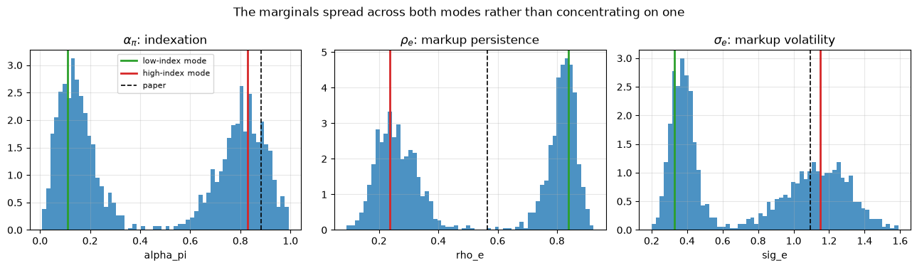
Fig. 139.1 Marginal posteriors for the parameters that separate the two modes#
The marginals are wide and lumpy rather than the tidy bells that every other parameter produces.
The chains do move between the two regions, but slowly, and that slow movement is precisely what the poor effective sample sizes were reporting.
Thirty thousand random walk draws never made the trip at all.
The economics behind the two modes is a familiar identification problem.
The data over 1960-1983 cannot tell us whether inflation is persistent because prices are indexed to past inflation or because the shocks pushing inflation around are themselves persistent.
Both stories fit, and the published estimates describe the one the data like slightly less.
139.14.8. Does the bimodality change the economics?#
This is the question that matters for the rest of the lecture.
h_mode_a = h_zero(unpack(v_mode_a))
h_mode_b = h_zero(unpack(v_mode))
print(f'h(0) at the low-indexation mode   {h_mode_a[0]:.4f}, {h_mode_a[1]:.4f}')
print(f'h(0) at the high-indexation mode  {h_mode_b[0]:.4f}, {h_mode_b[1]:.4f}')

h_nuts = np.array([h_zero(unpack(v)) for v in nuts_kept])
low = nuts_kept[:, FREE.index('alpha_pi')] < 0.5
print(f'\n{low.sum()} of {len(low)} NUTS draws sit on the low-indexation side')
for tag, m in [('low-indexation draws ', low), ('high-indexation draws', ~low)]:
    if m.sum() < 20:
        continue
    print(f'{tag}  h_pi {h_nuts[m, 0].mean():.4f} '
          f'[{np.percentile(h_nuts[m, 0], 5):.4f}, {np.percentile(h_nuts[m, 0], 95):.4f}]'
          f'   h_R {h_nuts[m, 1].mean():.4f} '
          f'[{np.percentile(h_nuts[m, 1], 5):.4f}, {np.percentile(h_nuts[m, 1], 95):.4f}]')
h(0) at the low-indexation mode   0.8632, 0.8292
h(0) at the high-indexation mode  0.9765, 0.7694

801 of 1600 NUTS draws sit on the low-indexation side
low-indexation draws   h_pi 0.8300 [0.7056, 0.9234]   h_R 0.8047 [0.6694, 0.9153]
high-indexation draws  h_pi 0.9624 [0.9017, 1.0014]   h_R 0.7816 [0.6403, 0.8990]
fig, axes = plt.subplots(1, 2, figsize=(11, 3.8))
for ax, j, ttl in zip(axes, [0, 1],
                      [r'$h_{\pi,\Delta m}(0)$', r'$h_{R,\Delta m}(0)$']):
    ax.hist(h_draws[:, j], bins=50, density=True, alpha=0.55,
            color='C0', label='RWMH')
    ax.hist(h_nuts[:, j], bins=50, density=True, alpha=0.55,
            color='C3', label='NUTS')
    ax.axvline(1, color='0.3', ls='--', lw=1.5)
    ax.set_title(ttl)
    ax.legend(fontsize=9)
fig.suptitle('The low-frequency slopes are robust across samplers and modes')
plt.tight_layout()
plt.show()
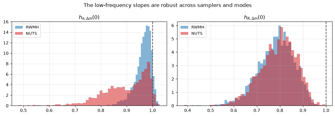
The reassuring answer is that it does not.
The two modes disagree sharply about why inflation is persistent and far less about the low-frequency slopes that this lecture is about.
Whether inflation persistence is intrinsic or inherited, \(h_{\pi,\Delta m}(0)\) stays between about four fifths and one, and \(h_{R,\Delta m}(0)\) sits near four fifths in both cases.
The paper’s substantive conclusions survive the discovery that its parameter estimates describe a local mode.
139.14.9. Comparing the samplers#
With that settled we can return to efficiency.
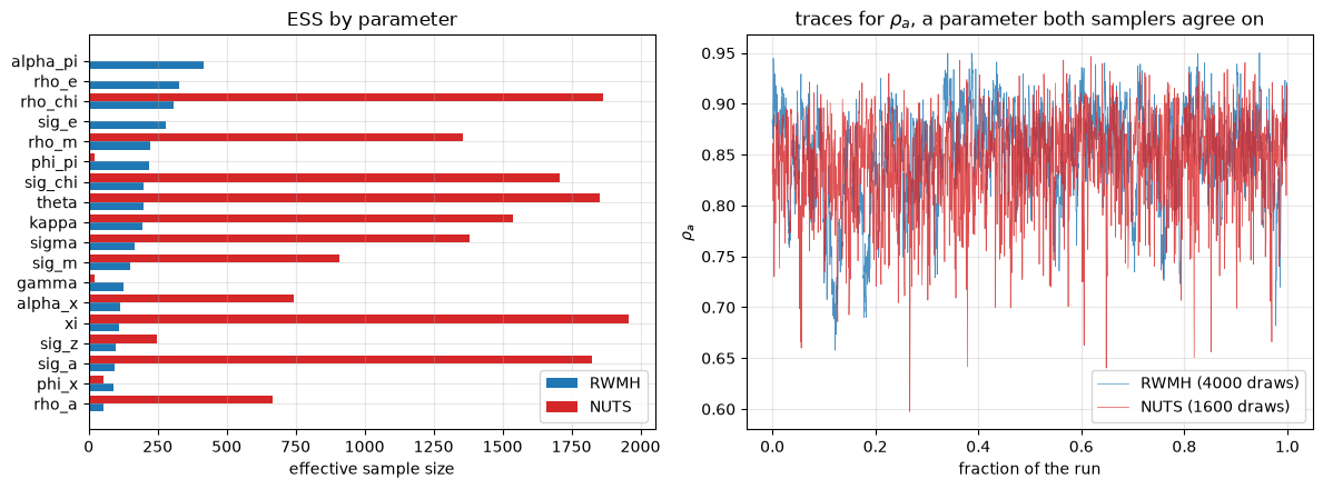
Effective sample sizes for the three parameters that separate the modes are not comparable across the two samplers, because for NUTS they partly measure movement between modes while for the random walk they measure movement within one.
We therefore compare medians rather than minima.
compare = pd.DataFrame({
    'RWMH mean': rwmh_summary['mean'], 'NUTS mean': nuts_summary['mean'],
    'RWMH ESS': rwmh_summary['ess_bulk'], 'NUTS ESS': nuts_summary['ess_bulk'],
    'NUTS r_hat': nuts_summary['r_hat']})
compare['ESS ratio'] = compare['NUTS ESS'] / compare['RWMH ESS']
compare.round(3)
| RWMH mean | NUTS mean | RWMH ESS | NUTS ESS | NUTS r_hat | ESS ratio | |
|---|---|---|---|---|---|---|
| theta | 0.989 | 0.989 | 197.674 | 1853.379 | 0.999 | 9.376 |
| alpha_pi | 0.816 | 0.476 | 415.958 | 6.208 | 1.737 | 0.015 |
| kappa | 0.117 | 0.109 | 195.344 | 1539.318 | 1.005 | 7.880 |
| alpha_x | 0.380 | 0.388 | 112.547 | 744.971 | 1.014 | 6.619 |
| sigma | 0.082 | 0.086 | 165.631 | 1381.327 | 1.008 | 8.340 |
| xi | 3.579 | 3.538 | 111.759 | 1955.615 | 1.003 | 17.498 |
| gamma | 2.043 | 1.920 | 125.072 | 21.332 | 1.134 | 0.171 |
| phi_pi | -0.236 | -0.367 | 220.898 | 20.459 | 1.143 | 0.093 |
| phi_x | -0.799 | -0.884 | 91.547 | 53.000 | 1.056 | 0.579 |
| rho_m | 0.516 | 0.515 | 221.684 | 1356.376 | 1.004 | 6.119 |
| rho_e | 0.258 | 0.539 | 328.990 | 6.220 | 1.732 | 0.019 |
| rho_a | 0.850 | 0.840 | 53.416 | 664.974 | 1.017 | 12.449 |
| rho_chi | 0.517 | 0.509 | 307.121 | 1865.524 | 1.006 | 6.074 |
| sig_e | 1.165 | 0.756 | 279.498 | 6.241 | 1.732 | 0.022 |
| sig_a | 0.247 | 0.248 | 93.286 | 1823.672 | 1.005 | 19.549 |
| sig_chi | 0.141 | 0.149 | 200.244 | 1706.324 | 1.001 | 8.521 |
| sig_z | 0.713 | 0.729 | 96.781 | 246.245 | 1.027 | 2.544 |
| sig_m | 0.714 | 0.723 | 149.238 | 908.919 | 1.015 | 6.090 |
unimodal = ~nuts_summary.index.isin(worst)
r_med = rwmh_summary['ess_bulk'][unimodal].median()
n_med = nuts_summary['ess_bulk'][unimodal].median()

print(f'{"":26s}{"RWMH":>12s}{"NUTS":>12s}')
print(f'{"draws kept":26s}{len(kept):12d}{len(nuts_kept):12d}')
print(f'{"seconds":26s}{rwmh_seconds:12.0f}{nuts_seconds:12.0f}')
print(f'{"median ESS":26s}{r_med:12.0f}{n_med:12.0f}')
print(f'{"median ESS per 1000 draws":26s}{1000 * r_med / len(kept):12.1f}'
      f'{1000 * n_med / len(nuts_kept):12.1f}')
print(f'{"median ESS per second":26s}{r_med / rwmh_seconds:12.2f}'
      f'{n_med / nuts_seconds:12.2f}')
print(f'\n{"speed-up in ESS per second":30s}'
      f'{(n_med / nuts_seconds) / (r_med / rwmh_seconds):6.1f}x')
                                  RWMH        NUTS
draws kept                        4000        1600
seconds                            275         345
median ESS                         149        1356
median ESS per 1000 draws         37.3       847.7
median ESS per second             0.54        3.93

speed-up in ESS per second       7.2x
Per draw the gap is very large, because each NUTS draw ends a trajectory that has travelled across the posterior rather than taking one small random step.
Cost claws some of that back, since a NUTS iteration needs many gradient evaluations where a random walk iteration needs one likelihood evaluation.
Effective draws per second is the ratio that matters, and it still favours NUTS by a wide margin.
139.14.10. What to take away#
The obstacle to Hamiltonian methods in DSGE estimation is the model solver, not the statistics.
Replacing an eigenvalue-sorting solver by a fixed point that uses only linear algebra buys exact gradients for about the cost of one extra likelihood evaluation, and that is enough to put NUTS within reach.
The payoff was not only speed.
Cheap chains made it cheap to run several of them and inspect their diagnostics, and the parameters that mixed worst pointed straight at a second and better mode that thirty thousand random walk draws had never visited.
Two caveats are worth stating.
First, the fixed point returns something meaningless where no stable solution exists, so a sampler that wanders outside the determinacy region will produce nonsense rather than a rejection; the posterior here sits well inside that region, but a flatter one might not.
Second, the efficiency gain reported above is specific to this posterior, and a well-scaled posterior in fewer dimensions would narrow the gap considerably.
139.15. Concluding remarks#
Lucas [1980] was careful to say that his two unit slopes should be expected to hold under some monetary policies and to break down under others.
Extending his sample by half a century confirms the breakdowns.
Estimating a small structural model on a sample like his, and then moving only the monetary policy rule, produces slopes that range over most of what the data display.
The lesson is the one Lucas, Sargent [1971], and Whiteman [1984] all drew, namely that low-frequency regression coefficients are not structural.
Working through the model from scratch adds something to the paper’s account.
Lucas’s first illustration, the unit slope of inflation on money growth, is an identity in this model whenever money growth is econometrically exogenous, because money demand is a quantity equation whose remaining terms are all first differences.
His second illustration, the unit slope of the interest rate on money growth, has no such support and moves around freely.
So the two illustrations, which look symmetric in a scatter plot, are quite different objects from the perspective of a structural model.
That asymmetry also marks the limit of the exercise, as Exercise 139.2 brings out.
Because \(h_{\pi,\Delta m}(0)\) is anchored at one by money demand, driving it to the near-zero values that the post-1984 data display takes a money growth rule far more anti-inflationary than the one those same data select.
On the computational side, the model turned out to be a useful test bed for Hamiltonian Monte Carlo.
The barrier to using it on DSGE models is not statistical but algorithmic: the standard solvers sort eigenvalues, and sorting has no derivative.
Swapping in a fixed-point solver that uses only linear algebra restores exact gradients, and the sampler that becomes available is far more efficient per unit of computing time on a posterior as badly scaled as this one.
The larger dividend was a diagnostic one.
Cheap chains and their convergence diagnostics led us to a second mode, and the posterior turned out to be bimodal: the data cannot choose between intrinsic and inherited inflation persistence, and the mode nearest the published estimates is the lower of the two.
That the two modes nonetheless agree about \(h_{\pi,\Delta m}(0)\) and \(h_{R,\Delta m}(0)\) is a piece of good news for the paper that only the more thorough sampler could deliver.
139.16. Exercises#
Exercise 139.1
The paper takes technology growth to be serially uncorrelated.
Replace \(z_t = \varepsilon_{zt}\) by \(z_t = \rho_z z_{t-1} + \varepsilon_{zt}\) and ask two questions.
Does Proposition 139.1 survive, and does persistent technology growth offer a route to breaking the unit slope that has nothing to do with monetary policy?
Solution
The technology block is row 7 of the canonical form, where g1[7, Z] is currently zero.
def canonical_rho_z(p, rule='money'):
    g0, g1, psi, pie = canonical(p, rule)
    g1[7, Z] = p['rho_z']
    return g0, g1, psi, pie


def h_zero_rho_z(p):
    G1, impact, eu = gensys(*canonical_rho_z(p))
    if eu != (1, 1):
        return np.nan, np.nan
    sd = np.diag([p['sig_e'], p['sig_a'], p['sig_chi'], p['sig_z'], p['sig_m']])
    n = NY + 2
    A, B = np.zeros((n, n)), np.zeros((n, 5))
    A[:NY, :NY], A[NY, X], A[NY + 1, A_] = G1, 1, 1
    B[:NY] = impact @ sd
    C = np.zeros((4, n))
    C[0, DM], C[1, PI], C[2, R], C[3, Z] = 1, 1, 1, 1
    C[3, X], C[3, NY] = 1, -1
    C[3, A_], C[3, NY + 1] = p['xi'], -p['xi']
    if np.max(np.abs(np.linalg.eigvals(A))) > 1 - 1e-9:
        return np.nan, np.nan
    return (h_zero_from_state_space(A, B, C, 1, 0),
            h_zero_from_state_space(A, B, C, 2, 0))


print('exogenous money growth, phi_pi = phi_x = 0')
for rho_z in [0.0, 0.3, 0.6, 0.9]:
    q = dict(p_bar, phi_pi=0.0, phi_x=0.0, rho_z=rho_z)
    print(f'   rho_z = {rho_z:.1f}:  h_pi = {h_zero_rho_z(q)[0]:.10f}, '
          f'h_R = {h_zero_rho_z(q)[1]:.4f}')

print('\nwith policy feedback, phi_pi = -2, phi_x = -0.5')
for rho_z in [0.0, 0.3, 0.6, 0.9]:
    q = dict(p_bar, phi_pi=-2.0, phi_x=-0.5, rho_z=rho_z)
    print(f'   rho_z = {rho_z:.1f}:  h_pi = {h_zero_rho_z(q)[0]:.4f}, '
          f'h_R = {h_zero_rho_z(q)[1]:.4f}')
exogenous money growth, phi_pi = phi_x = 0
   rho_z = 0.0:  h_pi = 1.0000000000, h_R = 0.4111
   rho_z = 0.3:  h_pi = 1.0000000000, h_R = 0.4111
   rho_z = 0.6:  h_pi = 1.0000000000, h_R = 0.4111
   rho_z = 0.9:  h_pi = 1.0000000000, h_R = 0.4111

with policy feedback, phi_pi = -2, phi_x = -0.5
   rho_z = 0.0:  h_pi = 0.4897, h_R = 0.7767
   rho_z = 0.3:  h_pi = 0.2340, h_R = 0.6392
   rho_z = 0.6:  h_pi = -0.1354, h_R = 0.3046
   rho_z = 0.9:  h_pi = -0.4584, h_R = -0.2820
Proposition 139.1 survives untouched, because its proof used only that technology is orthogonal to the policy shock, never how persistent it is.
Under exogenous money growth both slopes are invariant to \(\rho_z\), and for a reason worth noticing: \(z_t\) enters the model only contemporaneously, through money demand, so \(\rho_z\) changes the dynamics of technology without changing anyone’s response to a money shock.
Once policy feeds back the picture is different, and persistent technology growth pulls \(h_{\pi,\Delta m}(0)\) well away from one.
So the answer to the second question is yes, and it points at a limitation of the paper’s experiment: the technology process is held fixed while policy varies, but the two interact.
Exercise 139.2
The lecture estimates the model on 1960:I-1983:IV.
Find the posterior mode on 1984:I-2007:IV and compare the policy coefficients and the implied \(h(0)\) with what we found for the earlier sample.
The VAR put \(h_{\pi,\Delta m}(0)\) near zero over 1984-2007, so does the structural model, re-estimated, agree?
Solution
mask2 = (data.index.year >= 1984) & (data.index.year <= 2007)
Y2 = data.loc[mask2, VARS].values
Y2 = Y2 - Y2.mean(0)

res2 = optimize.minimize(lambda v: -log_post(v, Y2), v_mode, method='Powell',
                         options=dict(maxiter=20000, maxfev=20000))
res2 = optimize.minimize(lambda v: -log_post(v, Y2), res2.x, method='L-BFGS-B',
                         bounds=[SUPPORT[n] for n in FREE])
v2 = res2.x
print('                       1960-1983    1984-2007')
for n in ['phi_pi', 'phi_x', 'rho_m']:
    j = FREE.index(n)
    print(f'   {n:9s} {v_mode[j]:11.4f} {v2[j]:12.4f}')
print('   %-9s %5.3f, %.3f  %5.3f, %.3f'
      % (('model h(0)',) + h_zero(unpack(v_mode)) + h_zero(unpack(v2))))
for name, lo, hi in [('1960-1983', 1960, 1983), ('1984-2007', 1984, 2007)]:
    m = (data.index.year >= lo) & (data.index.year <= hi)
    med = np.nanmedian(bvar_h0(data.loc[m, VARS].values), axis=0)
    print(f'   VAR   h(0) on {name}: {med[0]:.3f}, {med[1]:.3f}')
                       1960-1983    1984-2007
   phi_pi        -0.1957      -0.0399
   phi_x         -0.5739      -1.5633
   rho_m          0.5301       0.3080
   model h(0) 0.976, 0.769  0.989, 0.858
   VAR   h(0) on 1960-1983: 0.739, 0.607
   VAR   h(0) on 1984-2007: -0.073, 0.268
The re-estimated model does not agree with the VAR.
The policy coefficients move, but the implied \(h_{\pi,\Delta m}(0)\) stays close to one on both samples, while the VAR puts it near zero after 1984.
Proposition 139.1 explains why this had to be hard.
Within this model \(h_{\pi,\Delta m}(0)\) is anchored at one and is dragged away from it only by policy feedback, so reaching values near zero needs a large negative \(\phi_\pi\), and the post-1984 data do not put the money growth rule anywhere near there.
That is a genuine tension between the paper’s Section II and its Section III: the contour plot shows a policy rule that could generate the low slopes, but the rule the later data actually select is not that rule.
A full comparison would run the sampler on both samples rather than compare modes.
Exercise 139.3
Figure 8 of the paper asks whether a fall in the variance of supply shocks, rather than a change in policy, could account for the decline in \(h(0)\).
Redo the money rule contour plot with \(\sigma_e\) cut to one quarter of its posterior mean and report how much the picture moves.
Solution
p_small_e = dict(p_bar, sig_e=p_bar['sig_e'] / 4)
Hpi2, HR2 = h_grid(p_small_e, 'money', 'phi_pi', 'phi_x',
                   phi_pi_grid, phi_x_grid)

print('baseline    h_pi in [%.2f, %.2f],  h_R in [%.2f, %.2f]'
      % (np.nanmin(Hpi), np.nanmax(Hpi), np.nanmin(HR), np.nanmax(HR)))
print('small sig_e h_pi in [%.2f, %.2f],  h_R in [%.2f, %.2f]'
      % (np.nanmin(Hpi2), np.nanmax(Hpi2), np.nanmin(HR2), np.nanmax(HR2)))
print('largest change in h_pi across the grid: %.3f'
      % np.nanmax(np.abs(Hpi2 - Hpi)))

contour_panel(phi_pi_grid, phi_x_grid, Hpi2, HR2, r'$\phi_\pi$', r'$\phi_x$',
              r'Low-frequency slopes with $\sigma_e$ cut to one quarter')
baseline    h_pi in [0.10, 1.06],  h_R in [0.06, 1.21]
small sig_e h_pi in [0.10, 1.06],  h_R in [0.06, 1.00]
largest change in h_pi across the grid: 0.432
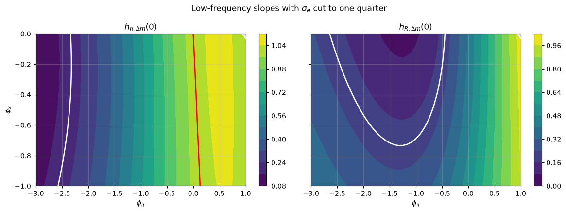
The range that \(h_{\pi,\Delta m}(0)\) can reach is unchanged, and the mapping from policy to \(h(0)\) keeps the same shape.
The contours do move within that range, by up to a few tenths at some grid points, so the claim is not that shock variances are irrelevant.
It is the weaker claim the paper makes, that a change in shock variances of this magnitude is not enough to substitute for a change in policy.