83. Cass-Koopmans Competitive Equilibrium#
83.1. Overview#
This lecture continues our analysis in this lecture Cass-Koopmans Planning Model about the model that Tjalling Koopmans [Koopmans, 1965] and David Cass [Cass, 1965] used to study optimal capital accumulation.
This lecture illustrates what is, in fact, a more general connection between a planned economy and an economy organized as a competitive equilibrium or a market economy.
The earlier lecture Cass-Koopmans Planning Model studied a planning problem and used ideas including
A Lagrangian formulation of the planning problem that leads to a system of difference equations.
A shooting algorithm for solving difference equations subject to initial and terminal conditions.
A turnpike property that describes optimal paths for long-but-finite horizon economies.
The present lecture uses additional ideas including
Hicks-Arrow prices, named after John R. Hicks and Kenneth Arrow.
A connection between some Lagrange multipliers from the planning problem and the Hicks-Arrow prices.
A Big \(K\) , little \(k\) trick widely used in macroeconomic dynamics.
We shall encounter this trick in this lecture and also in this lecture.
A non-stochastic version of a theory of the term structure of interest rates.
An intimate connection between two ways to organize an economy, namely:
socialism in which a central planner commands the allocation of resources, and
competitive markets in which competitive equilibrium prices induce individual consumers and producers to choose a socially optimal allocation as unintended consequences of their selfish decisions
Let’s start with some standard imports:
import matplotlib.pyplot as plt
from numba import jit, float64
from numba.experimental import jitclass
import numpy as np
83.2. Review of Cass-Koopmans Model#
The physical setting is identical with that in Cass-Koopmans Planning Model.
Time is discrete and takes values \(t = 0, 1 , \ldots, T\).
Output of a single good can either be consumed or invested in physical capital.
The capital good is durable but partially depreciates each period at a constant rate.
We let \(C_t\) be a nondurable consumption good at time t.
Let \(K_t\) be the stock of physical capital at time t.
Let \(\vec{C}\) = \(\{C_0,\dots, C_T\}\) and \(\vec{K}\) = \(\{K_0,\dots,K_{T+1}\}\).
A representative household is endowed with one unit of labor at each \(t\) and likes the consumption good at each \(t\).
The representative household inelastically supplies a single unit of labor \(N_t\) at each \(t\), so that \(N_t =1 \text{ for all } t \in \{0, 1, \ldots, T\}\).
The representative household has preferences over consumption bundles ordered by the utility functional:
where \(\beta \in (0,1)\) is a discount factor and \(\gamma >0\) governs the curvature of the one-period utility function.
We assume that \(K_0 > 0\).
There is an economy-wide production function
with \(0 < \alpha<1\), \(A > 0\).
A feasible allocation \(\vec{C}, \vec{K}\) satisfies
where \(\delta \in (0,1)\) is a depreciation rate of capital.
83.2.1. Planning Problem#
In this lecture Cass-Koopmans Planning Model, we studied a problem in which a planner chooses an allocation \(\{\vec{C},\vec{K}\}\) to maximize (82.2) subject to (82.5).
The allocation that solves the planning problem reappears in a competitive equilibrium, as we shall see below.
83.3. Competitive Equilibrium#
We now study a decentralized version of the economy.
It shares the same technology and preference structure as the planned economy studied in this lecture Cass-Koopmans Planning Model.
But now there is no planner.
There are (unit masses of) price-taking consumers and firms.
Market prices are set to reconcile distinct decisions that are made separately by a representative consumer and a representative firm.
There is a representative consumer who has the same preferences over consumption plans as did a consumer in the planned economy.
Instead of being told what to consume and save by a planner, a consumer (also known as a household) chooses for itself subject to a budget constraint.
At each time \(t\), the consumer receives wages and rentals of capital from a firm – these comprise its income at time \(t\).
The consumer decides how much income to allocate to consumption or to savings.
The household can save either by acquiring additional physical capital (it trades one for one with time \(t\) consumption) or by acquiring claims on consumption at dates other than \(t\).
The household owns physical capital and labor and rents them to the firm.
The household consumes, supplies labor, and invests in physical capital.
A profit-maximizing representative firm operates the production technology.
The firm rents labor and capital each period from the representative household and sells its output each period to the household.
The representative household and the representative firm are both price takers who believe that prices are not affected by their choices
Note
Again, we can think of there being unit measures of identical representative consumers and identical representative firms.
83.4. Market Structure#
The representative household and the representative firm are both price takers.
The household owns both factors of production, namely, labor and physical capital.
Each period, the firm rents both factors from the household.
There is a single grand competitive market in which a household trades date \(0\) goods for goods at all other dates \(t=1, 2, \ldots, T\).
83.4.1. Prices#
There are sequences of prices \(\{w_t,\eta_t\}_{t=0}^T= \{\vec{w}, \vec{\eta} \}\) where
\(w_t\) is a wage, i.e., a rental rate, for labor at time \(t\)
\(\eta_t\) is a rental rate for capital at time \(t\)
In addition there is a vector \(\{q_t^0\}\) of intertemporal prices where
\(q^0_t\) is the price at time \(0\) of one unit of the good at date \(t\).
We call \(\{q^0_t\}_{t=0}^T\) a vector of Hicks-Arrow prices, named after the 1972 economics Nobel prize winners.
Because is a relative price. the unit of account in terms of which the prices \(q^0_t\) are stated is; we are free to re-normalize them by multiplying all of them by a positive scalar, say \(\lambda > 0\).
Units of \(q_t^0\) could be set so that they are
In this case, we would be taking the time \(0\) consumption good to be the numeraire.
83.5. Firm Problem#
At time \(t\) a representative firm hires labor \(\tilde n_t\) and capital \(\tilde k_t\).
The firm’s profits at time \(t\) are
where \(w_t\) is a wage rate at \(t\) and \(\eta_t\) is the rental rate on capital at \(t\).
As in the planned economy model
83.5.1. Zero Profit Conditions#
Zero-profits conditions for capital and labor are
and
These conditions emerge from a no-arbitrage requirement.
To describe this no-arbitrage profits reasoning, we begin by applying a theorem of Euler about linearly homogenous functions.
The theorem applies to the Cobb-Douglas production function because we it displays constant returns to scale:
for \(\alpha \in (0,1)\).
Taking partial derivatives \(\frac{\partial }{\partial \alpha}\) on both sides of the above equation gives
Rewrite the firm’s profits as
or
Because \(F\) is homogeneous of degree \(1\), it follows that \(\frac{\partial F}{\partial \tilde k_t}\) and \(\frac{\partial F}{\partial \tilde n_t}\) are homogeneous of degree \(0\) and therefore fixed with respect to \(\tilde k_t\) and \(\tilde n_t\).
If \(\frac{\partial F}{\partial \tilde k_t}> \eta_t\), then the firm makes positive profits on each additional unit of \(\tilde k_t\), so it would want to make \(\tilde k_t\) arbitrarily large.
But setting \(\tilde k_t = + \infty\) is not physically feasible, so equilibrium prices must take values that present the firm with no such arbitrage opportunity.
A similar argument applies if \(\frac{\partial F}{\partial \tilde n_t}> w_t\).
If \(\frac{\partial \tilde k_t}{\partial \tilde k_t}< \eta_t\), the firm would want to set \(\tilde k_t\) to zero, which is not feasible.
It is convenient to define \(\vec{w} =\{w_0, \dots,w_T\}\) and \(\vec{\eta}= \{\eta_0, \dots, \eta_T\}\).
83.6. Household Problem#
A representative household lives at \(t=0,1,\dots, T\).
At \(t\), the household rents \(1\) unit of labor and \(k_t\) units of capital to a firm and receives income
At \(t\) the household allocates its income to the following purchases between the following two categories:
consumption \(c_t\)
net investment \(k_{t+1} -(1-\delta)k_t\)
Here \(\left(k_{t+1} -(1-\delta)k_t\right)\) is the household’s net investment in physical capital and \(\delta \in (0,1)\) is again a depreciation rate of capital.
In period \(t\), the consumer is free to purchase more goods to be consumed and invested in physical capital than its income from supplying capital and labor to the firm, provided that in some other periods its income exceeds its purchases.
A consumer’s net excess demand for time \(t\) consumption goods is the gap
Let \(\vec{c} = \{c_0,\dots,c_T\}\) and let \(\vec{k} = \{k_1,\dots,k_{T+1}\}\).
\(k_0\) is given to the household.
The household faces a single budget constraint that requires that the present value of the household’s net excess demands must be zero:
or
The household faces price system \(\{q^0_t, w_t, \eta_t\}\) as a price-taker and chooses an allocation to solve the constrained optimization problem:
Components of a price system have the following units:
\(w_t\) is measured in units of the time \(t\) good per unit of time \(t\) labor hired
\(\eta_t\) is measured in units of the time \(t\) good per unit of time \(t\) capital hired
\(q_t^0\) is measured in units of a numeraire per unit of the time \(t\) good
83.6.1. Definitions#
A price system is a sequence \(\{q_t^0,\eta_t,w_t\}_{t=0}^T= \{\vec{q}, \vec{\eta}, \vec{w}\}\).
An allocation is a sequence \(\{c_t,k_{t+1},n_t=1\}_{t=0}^T = \{\vec{c}, \vec{k}, \vec{n}\}\).
A competitive equilibrium is a price system and an allocation with the following properties:
Given the price system, the allocation solves the household’s problem.
Given the price system, the allocation solves the firm’s problem.
The vision here is that an equilibrium price system and allocation are determined once and for all.
In effect, we imagine that all trades occur just before time \(0\).
83.7. Computing a Competitive Equilibrium#
We compute a competitive equilibrium by using a guess and verify approach.
We guess equilibrium price sequences \(\{\vec{q}, \vec{\eta}, \vec{w}\}\).
We then verify that at those prices, the household and the firm choose the same allocation.
83.7.1. Guess for Price System#
In this lecture Cass-Koopmans Planning Model, we computed an allocation \(\{\vec{C}, \vec{K}, \vec{N}\}\) that solves a planning problem.
We use that allocation to construct a guess for the equilibrium price system.
Note
This allocation will constitute the Big \(K\) to be in the present instance of the Big \(K\) , little \(k\) trick that we’ll apply to a competitive equilibrium in the spirit of this lecture and this lecture.
In particular, we shall use the following procedure:
obtain first-order conditions for the representative firm and the representative consumer.
from these equations, obtain a new set of equations by replacing the firm’s choice variables \(\tilde k, \tilde n\) and the consumer’s choice variables with the quantities \(\vec C, \vec K\) that solve the planning problem.
solve the resulting equations for \(\{\vec{q}, \vec{\eta}, \vec{w}\}\) as functions of \(\vec C, \vec K\).
verify that at these prices, \(c_t = C_t, k_t = \tilde k_t = K_t, \tilde n_t = 1\) for \(t = 0, 1, \ldots, T\).
Thus, we guess that for \(t=0,\dots,T\):
At these prices, let capital chosen by the household be
and let the allocation chosen by the firm be
and so on.
If our guess for the equilibrium price system is correct, then it must occur that
We shall verify that for \(t=0,\dots,T\) allocations chosen by the household and the firm both equal the allocation that solves the planning problem:
83.7.2. Verification Procedure#
Our approach is firsts to stare at first-order necessary conditions for optimization problems of the household and the firm.
At the price system we have guessed, we’ll then verify that both sets of first-order conditions are satisfied at the allocation that solves the planning problem.
83.7.3. Household’s Lagrangian#
To solve the household’s problem, we formulate the Lagrangian
and attack the min-max problem:
First-order conditions are
Now we plug in our guesses of prices and do some algebra in the hope of recovering all first-order necessary conditions (82.9)-(82.12) for the planning problem from this lecture Cass-Koopmans Planning Model.
Combining (83.9) and (83.2), we get:
which is (82.9).
Combining (83.10), (83.2), and (83.4), we get:
Rewriting (83.13) by dividing by \(\lambda\) on both sides (which is nonzero since u’>0) we get:
or
which is (82.10).
Combining (83.11), (83.2), (83.3) and (83.4) after multiplying both sides of (83.11) by \(\lambda\), we get
which simplifies to
Since \(\beta^t \mu_t >0\) for \(t =0, \ldots, T\), it follows that
which is (82.11).
Combining (83.12) and (83.2), we get:
Dividing both sides by \(\beta^{T+1}\) gives
which is (82.12) for the planning problem.
Thus, at our guess of the equilibrium price system, the allocation that solves the planning problem also solves the problem faced by a representative household living in a competitive equilibrium.
83.7.4. Representative Firm’s Problem#
We now turn to the problem faced by a firm in a competitive equilibrium:
If we plug (83.8) into (83.1) for all t, we get
which is (83.4).
If we now plug (83.8) into (83.1) for all t, we get:
which is exactly (83.5).
Thus, at our guess for the equilibrium price system, the allocation that solves the planning problem also solves the problem faced by a firm within a competitive equilibrium.
By (83.6) and (83.7) this allocation is identical to the one that solves the consumer’s problem.
Note
Because budget sets are affected only by relative prices, \(\{q^0_t\}\) is determined only up to multiplication by a positive constant.
Normalization: We are free to choose a \(\{q_t^0\}\) that makes \(\lambda=1\) so that we are measuring \(q_t^0\) in units of the marginal utility of time \(0\) goods.
We will plot \(q, w, \eta\) below to show these equilibrium prices induce the same aggregate movements that we saw earlier in the planning problem.
To proceed, we bring in Python code that Cass-Koopmans Planning Model used to solve the planning problem
First let’s define a jitclass that stores parameters and functions
the characterize an economy.
planning_data = [
    ('γ', float64),    # Coefficient of relative risk aversion
    ('β', float64),    # Discount factor
    ('δ', float64),    # Depreciation rate on capital
    ('α', float64),    # Return to capital per capita
    ('A', float64)     # Technology
]
@jitclass(planning_data)
class PlanningProblem():

    def __init__(self, γ=2, β=0.95, δ=0.02, α=0.33, A=1):

        self.γ, self.β = γ, β
        self.δ, self.α, self.A = δ, α, A

    def u(self, c):
        '''
        Utility function
        ASIDE: If you have a utility function that is hard to solve by hand
        you can use automatic or symbolic differentiation
        See https://github.com/HIPS/autograd
        '''
        γ = self.γ

        return c ** (1 - γ) / (1 - γ) if γ!= 1 else np.log(c)

    def u_prime(self, c):
        'Derivative of utility'
        γ = self.γ

        return c ** (-γ)

    def u_prime_inv(self, c):
        'Inverse of derivative of utility'
        γ = self.γ

        return c ** (-1 / γ)

    def f(self, k):
        'Production function'
        α, A = self.α, self.A

        return A * k ** α

    def f_prime(self, k):
        'Derivative of production function'
        α, A = self.α, self.A

        return α * A * k ** (α - 1)

    def f_prime_inv(self, k):
        'Inverse of derivative of production function'
        α, A = self.α, self.A

        return (k / (A * α)) ** (1 / (α - 1))

    def next_k_c(self, k, c):
        ''''
        Given the current capital Kt and an arbitrary feasible
        consumption choice Ct, computes Kt+1 by state transition law
        and optimal Ct+1 by Euler equation.
        '''
        β, δ = self.β, self.δ
        u_prime, u_prime_inv = self.u_prime, self.u_prime_inv
        f, f_prime = self.f, self.f_prime

        k_next = f(k) + (1 - δ) * k - c
        c_next = u_prime_inv(u_prime(c) / (β * (f_prime(k_next) + (1 - δ))))

        return k_next, c_next
@jit
def shooting(pp, c0, k0, T=10):
    '''
    Given the initial condition of capital k0 and an initial guess
    of consumption c0, computes the whole paths of c and k
    using the state transition law and Euler equation for T periods.
    '''
    if c0 > pp.f(k0):
        print("initial consumption is not feasible")

        return None

    # initialize vectors of c and k
    c_vec = np.empty(T+1)
    k_vec = np.empty(T+2)

    c_vec[0] = c0
    k_vec[0] = k0

    for t in range(T):
        k_vec[t+1], c_vec[t+1] = pp.next_k_c(k_vec[t], c_vec[t])

    k_vec[T+1] = pp.f(k_vec[T]) + (1 - pp.δ) * k_vec[T] - c_vec[T]

    return c_vec, k_vec
@jit
def bisection(pp, c0, k0, T=10, tol=1e-4, max_iter=500, k_ter=0, verbose=True):

    # initial boundaries for guess c0
    c0_upper = pp.f(k0)
    c0_lower = 0

    i = 0
    while True:
        c_vec, k_vec = shooting(pp, c0, k0, T)
        error = k_vec[-1] - k_ter

        # check if the terminal condition is satisfied
        if np.abs(error) < tol:
            if verbose:
                print('Converged successfully on iteration ', i+1)
            return c_vec, k_vec

        i += 1
        if i == max_iter:
            if verbose:
                print('Convergence failed.')
            return c_vec, k_vec

        # if iteration continues, updates boundaries and guess of c0
        if error > 0:
            c0_lower = c0
        else:
            c0_upper = c0

        c0 = (c0_lower + c0_upper) / 2
pp = PlanningProblem()

# Steady states
ρ = 1 / pp.β - 1
k_ss = pp.f_prime_inv(ρ+pp.δ)
c_ss = pp.f(k_ss) - pp.δ * k_ss
The above code from this lecture Cass-Koopmans Planning Model lets us compute an optimal allocation for the planning problem.
from the preceding analysis, we know that it will also be an allocation associated with a competitive equilibium.
Now we’re ready to bring in Python code that we require to compute additional objects that appear in a competitive equilibrium.
@jit
def q(pp, c_path):
    # Here we choose numeraire to be u'(c_0) -- this is q^(t_0)_t
    T = len(c_path) - 1
    q_path = np.ones(T+1)
    q_path[0] = 1
    for t in range(1, T+1):
        q_path[t] = pp.β ** t * pp.u_prime(c_path[t])
    return q_path

@jit
def w(pp, k_path):
    w_path = pp.f(k_path) - k_path * pp.f_prime(k_path)
    return w_path

@jit
def η(pp, k_path):
    η_path = pp.f_prime(k_path)
    return η_path
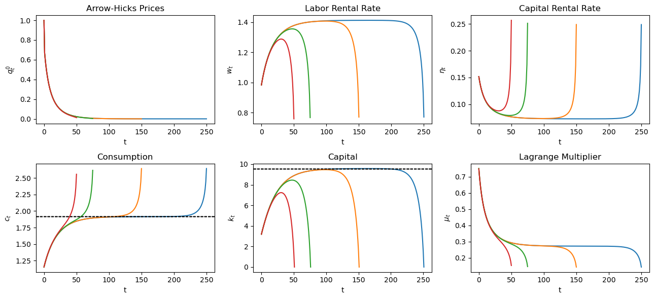
Now we calculate and plot for each \(T\)
T_arr = [250, 150, 75, 50]

fix, axs = plt.subplots(2, 3, figsize=(13, 6))
titles = ['Arrow-Hicks Prices', 'Labor Rental Rate', 'Capital Rental Rate',
          'Consumption', 'Capital', 'Lagrange Multiplier']
ylabels = ['$q_t^0$', '$w_t$', r'$\eta_t$', '$c_t$', '$k_t$', r'$\mu_t$']

for T in T_arr:
    c_path, k_path = bisection(pp, 0.3, k_ss/3, T, verbose=False)
    μ_path = pp.u_prime(c_path)

    q_path = q(pp, c_path)
    w_path = w(pp, k_path)[:-1]
    η_path = η(pp, k_path)[:-1]
    paths = [q_path, w_path, η_path, c_path, k_path, μ_path]

    for i, ax in enumerate(axs.flatten()):
        ax.plot(paths[i])
        ax.set(title=titles[i], ylabel=ylabels[i], xlabel='t')
        if titles[i] == 'Capital':
            ax.axhline(k_ss, lw=1, ls='--', c='k')
        if titles[i] == 'Consumption':
            ax.axhline(c_ss, lw=1, ls='--', c='k')

plt.tight_layout()
plt.show()
83.7.4.1. Varying Curvature#
Now we see how our results change if we keep \(T\) constant, but allow the curvature parameter, \(\gamma\) to vary, starting with \(K_0\) below the steady state.
We plot the results for \(T=150\)
T = 150
γ_arr = [1.1, 4, 6, 8]

fix, axs = plt.subplots(2, 3, figsize=(13, 6))

for γ in γ_arr:
    pp_γ = PlanningProblem(γ=γ)
    c_path, k_path = bisection(pp_γ, 0.3, k_ss/3, T, verbose=False)
    μ_path = pp_γ.u_prime(c_path)

    q_path = q(pp_γ, c_path)
    w_path = w(pp_γ, k_path)[:-1]
    η_path = η(pp_γ, k_path)[:-1]
    paths = [q_path, w_path, η_path, c_path, k_path, μ_path]

    for i, ax in enumerate(axs.flatten()):
        ax.plot(paths[i], label=fr'$\gamma = {γ}$')
        ax.set(title=titles[i], ylabel=ylabels[i], xlabel='t')
        if titles[i] == 'Capital':
            ax.axhline(k_ss, lw=1, ls='--', c='k')
        if titles[i] == 'Consumption':
            ax.axhline(c_ss, lw=1, ls='--', c='k')

axs[0, 0].legend()
plt.tight_layout()
plt.show()
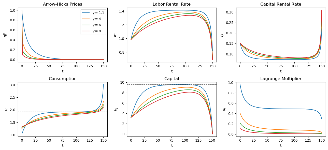
Adjusting \(\gamma\) means adjusting how much individuals prefer to smooth consumption.
Higher \(\gamma\) means individuals prefer to smooth more resulting in slower convergence to a steady state allocation.
Lower \(\gamma\) means individuals prefer to smooth less, resulting in faster convergence to a steady state allocation.
83.8. Yield Curves and Hicks-Arrow Prices#
We return to Hicks-Arrow prices and calculate how they are related to yields on loans of alternative maturities.
This will let us plot a yield curve that graphs yields on bonds of maturities \(j=1, 2, \ldots\) against \(j=1,2, \ldots\).
We use the following formulas.
A yield to maturity on a loan made at time \(t_0\) that matures at time \(t > t_0\)
A Hicks-Arrow price system for a base-year \(t_0\leq t\) satisfies
We redefine our function for \(q\) to allow arbitrary base years, and define a new function for \(r\), then plot both.
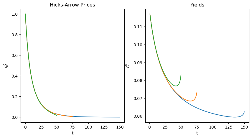
We begin by continuing to assume that \(t_0=0\) and plot things for different maturities \(t=T\), with \(K_0\) below the steady state
@jit
def q_generic(pp, t0, c_path):
    # simplify notations
    β = pp.β
    u_prime = pp.u_prime

    T = len(c_path) - 1
    q_path = np.zeros(T+1-t0)
    q_path[0] = 1
    for t in range(t0+1, T+1):
        q_path[t-t0] = β ** (t-t0) * u_prime(c_path[t]) / u_prime(c_path[t0])
    return q_path

@jit
def r(pp, t0, q_path):
    '''Yield to maturity'''
    r_path = - np.log(q_path[1:]) / np.arange(1, len(q_path))
    return r_path

def plot_yield_curves(pp, t0, c0, k0, T_arr):

    fig, axs = plt.subplots(1, 2, figsize=(10, 5))

    for T in T_arr:
        c_path, k_path = bisection(pp, c0, k0, T, verbose=False)
        q_path = q_generic(pp, t0, c_path)
        r_path = r(pp, t0, q_path)

        axs[0].plot(range(t0, T+1), q_path)
        axs[0].set(xlabel='t', ylabel='$q_t^0$', title='Hicks-Arrow Prices')

        axs[1].plot(range(t0+1, T+1), r_path)
        axs[1].set(xlabel='t', ylabel='$r_t^0$', title='Yields')
T_arr = [150, 75, 50]
plot_yield_curves(pp, 0, 0.3, k_ss/3, T_arr)
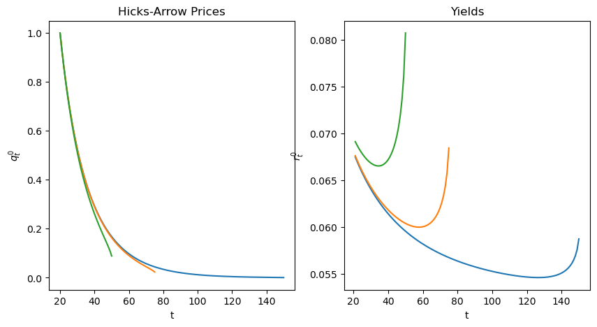
Now we plot when \(t_0=20\)
plot_yield_curves(pp, 20, 0.3, k_ss/3, T_arr)