127. Linear Quadratic Mean Field Games: Extensions#
127.1. Overview#
This lecture continues Linear Quadratic Mean Field Games, and it assumes familiarity with that lecture’s theory, through the split into individual and aggregate dynamics, and with its capital accumulation example.
There we studied a continuum of agents whose quadratic payoffs depend on the cross-sectional averages of states and actions, and found that equilibrium aggregate dynamics solve the Riccati equation of a single-agent problem in which strategic interaction changes only the curvatures.
Here we take up three extensions developed by Alvarez and Argente [2026]:
Cross terms between states and actions. The equivalence result survives when the mixed interactions between states and actions satisfy a symmetry restriction, with the mixed interaction subtracted from the own cross term, and uniqueness can fail when they do not.
Forcing processes. States that agents cannot control, such as costs, can be added without changing the Riccati equation of the controlled block, and a pricing example shows that firms pass idiosyncratic and common cost shocks through at different speeds and to different extents.
Higher moments. When payoffs depend on higher moments of the cross-sectional distribution, idiosyncratic risk affects aggregate persistence.
Let’s start with some imports:
import numpy as np
import matplotlib.pyplot as plt
from scipy.linalg import solve_continuous_are, expm
127.2. What we need from the previous lecture#
Throughout, lower-case letters denote an agent’s own state \(x\) and action \(\alpha\), and upper-case or calligraphic letters denote their cross-sectional averages \(X\) and \(\mathcal A\).
In Linear Quadratic Mean Field Games an agent has period return and state equation
and discounts at rate \(\rho\).
Given the aggregate paths, her value function is \(u(x,t) = \beta_0(t) + \beta_1(t)^\top x + \tfrac12 x^\top\bar\beta_2 x\), where \(\bar\beta_2\) solves the single-agent Riccati equation and involves neither interaction matrix.
In equilibrium the aggregate state follows \(\dot X = \left(B(\Gamma+\Theta_{\mathcal A})^{-1}B^\top P - A\right)X\), where the symmetric matrix \(P\) solves
and the eigenvalues of the closed-loop matrix must have real parts below \(\rho/2\).
That equation comes from a state-costate system whose eigenvalues come in pairs \(\lambda\) and \(\rho - \lambda\), so at most half of them lie below \(\rho/2\); with \(B(\Gamma + \Theta_{\mathcal A})^{-1}B^\top\) positive definite, that is what makes the equilibrium unique.
An agent’s deviation from the cross-sectional mean, \(z = x - X\), follows \(dz = (B\Gamma^{-1}B^\top\bar\beta_2 - A)z\,dt + \Sigma^{1/2}dW\), in which no interaction matrix appears.
So data on deviations from the mean contain no information about strategic interaction, which is the missing intercept.
Shocks common to all agents, modeled with a compensated jump process \(\mathcal J\), enter the law of motion of \(X\) but leave \(P\) unchanged.
We reuse two tools: the closed form for the aggregate eigenvalue in the scalar case,
and the calibration of the capital accumulation example.
In that example a firm with capital \(k\) earns \(\Pi(k, K) = k^{\nu(1-1/\eta)}K^{\nu/\eta}\) when the rest of the industry holds \(K\), pays an adjustment cost \(\psi(i) = \frac\phi2\bar i\left(\frac{i - \bar i}{\bar i}\right)^2\), and buys investment goods at price \(\mathcal P(I) = (I/\bar i)^{1/\varepsilon_s}\).
In percentage deviations from the steady state it maps into the scalar model with \(a = b = \delta\), \(q + \theta_X = \frac{\eta-1}{\eta}\nu(1-\nu)\), \(\gamma = \phi\,\delta\bar k^{1-\nu}\) and \(\theta_{\mathcal A} = \delta\bar k^{1-\nu}/\varepsilon_s\), and the calibration gives half-lives of three years for a firm’s deviation from the industry mean and five years for the industry.
def scalar_λ(ρ, a, b, q, γ, θ_X, θ_A):
    "Closed-form aggregate eigenvalue in the scalar case."
    return ρ/2 - np.sqrt((ρ/2 + a)**2 + b**2*(q + θ_X)/(γ + θ_A))

def half_life(λ):
    "Time for a state with eigenvalue λ < 0 to close half of a gap."
    return np.log(2)/(-λ)

def cap_q(η, ν):
    "Own-state curvature in the capital accumulation example."
    return ν*(η - 1)/η**2*(η*(1 - ν) + ν)

def cap_θ_X(η, ν):
    "State interaction in the capital accumulation example."
    return -(η - 1)/η*ν**2/η

ρ_c, δ_c, η_c, ν_c = 0.05, 0.10, 4.0, 0.7
φ_c, ε_s_c = 1/7, 35/9

def cap_scale(η, ν, ρ=ρ_c, δ=δ_c):
    "δ k̄^{1-ν}, which converts φ and 1/ε_s into γ and θ_A."
    return δ*ν*(η - 1)/(η*(ρ + δ))

γ_c = φ_c*cap_scale(η_c, ν_c)
θ_A_c = cap_scale(η_c, ν_c)/ε_s_c
q_c, θ_X_c = cap_q(η_c, ν_c), cap_θ_X(η_c, ν_c)

λ_c = scalar_λ(ρ_c, δ_c, δ_c, q_c, γ_c, θ_X_c, θ_A_c)          # industry
λ_micro = scalar_λ(ρ_c, δ_c, δ_c, q_c, γ_c, 0.0, 0.0)          # single firm
print(f"γ = {γ_c:.3f}, θ_A = {θ_A_c:.3f}")
print(f"half-lives: firm {half_life(λ_micro):.2f} years, industry {half_life(λ_c):.2f} years")
γ = 0.050, θ_A = 0.090
half-lives: firm 3.00 years, industry 4.99 years
127.3. State-action cross terms#
The return in Linear Quadratic Mean Field Games was not the most general quadratic return.
A second-order approximation to a general period return produces
The previous lecture used the first line throughout, and the terms in the aggregates alone in the third line when it studied the planner.
Here we restore the second line.
The own cross term \(C\) links an agent’s state and action.
It appears when adjustment costs depend on the state as well as on the action, as with investment costs that depend on the investment rate [Cooper and Haltiwanger, 2006, Hayashi, 1982].
The mixed interactions appear when the average state affects the marginal return to an agent’s action (\(\Theta_{X\alpha}\)), or the average action affects the marginal return to her state (\(\Theta_{x\mathcal A}\)).
127.3.1. The individual problem#
Taking the aggregate paths as given, the agent’s first-order condition is now
and the curvature of her value function solves
The own cross term enters the individual’s curvature, but, as before, no interaction matrix does.
Completing the square in the action,
shows that the counterpart of \(Q \succ 0\) is \(Q - C\Gamma^{-1}C^\top \succ 0\), which we assume.
127.3.2. The equilibrium#
Aggregating the first-order condition gives
It is convenient to track \(w \equiv \beta_1 + \bar\beta_2 X\), the marginal value of the state for an agent at the mean.
Differentiating, aggregating, and using (127.2) gives the state-costate system
The costate equation involves \(\Theta_{x\mathcal A}\), through which the average action shifts the marginal value of an agent’s state.
The aggregate action involves \(\Theta_{X\alpha}\), through which the average state shifts the marginal return to her action.
The two need not be equal, but when they are, the system keeps the Hamiltonian structure of the benchmark.
Proposition 127.1
Suppose \(\Theta_{X\alpha} = \Theta_{x\mathcal A}\), and write \(\tilde C \equiv C - \Theta_{X\alpha}\).
An equilibrium is characterized by a symmetric matrix \(P\) solving
with aggregate dynamics
This is the Riccati equation of a single agent whose return is
If \(\Gamma + \Theta_{\mathcal A} \succ 0\) and \(Q + \Theta_X - \tilde C(\Gamma + \Theta_{\mathcal A})^{-1}\tilde C^\top \succ 0\), an equilibrium exists and is unique.
So the equivalence result of Linear Quadratic Mean Field Games survives, with one more adjustment: the mixed interaction shifts the effective cross term from \(C\) to \(C - \Theta_{X\alpha}\).
Completing the square in the effective problem shows that a cross term does two things.
It lowers the effective state curvature to \(Q + \Theta_X - \tilde C(\Gamma+\Theta_{\mathcal A})^{-1}\tilde C^\top\), and it changes the effective drift matrix from \(A\) to \(A - B(\Gamma+\Theta_{\mathcal A})^{-1}\tilde C^\top\).
The comparative statics of the previous lecture apply to these transformed objects rather than to the interaction matrices themselves.
The dynamics of an agent’s deviation from the mean become
which involve the own cross term \(C\) but still no interaction matrix, so data on deviations from the mean still contain no information about strategic interaction.
The planner is handled in the same way.
Its effective cross term is \(C - \Theta_{X\alpha} - \Theta_{x\mathcal A} - \Lambda_{X\mathcal A}\), so it needs no restriction on the mixed interactions, which enter only through their sum.
To compute equilibria with cross terms, we extend the solver of Linear Quadratic Mean Field Games.
The s argument of solve_continuous_are replaces \(\tilde P B\) by \(\tilde P B + s\) in the quadratic term of the standard Riccati equation, so setting \(s = -\tilde C\) handles an effective cross term \(\tilde C\).
As in the previous lecture, the function checks the Riccati residual and the eigenvalue condition, and raises an error if either fails.
def closed_loop(A, B, Γ_eff, P, C=None):
    "The matrix governing aggregate dynamics, Ẋ = (B Γ_eff^{-1} (B' P + C') - A) X."
    K = B.T @ P if C is None else B.T @ P + C.T
    return B @ np.linalg.solve(Γ_eff, K) - A

def mfg_riccati(A, B, Q, Γ, ρ, C=None, tol=1e-8):
    """
    Solve  (P B + C) Γ^{-1} (B' P + C') = Q + ρ P + P A + A' P, with C = 0 by
    default, for the solution P whose closed-loop matrix has eigenvalues with
    real parts below ρ/2, and raise ValueError if there is none.
    """
    n, k = B.shape
    C_use = np.zeros((n, k)) if C is None else C
    try:
        P = -solve_continuous_are(-(A + ρ/2 * np.eye(n)), B, Q, Γ, s=-C_use)
    except (np.linalg.LinAlgError, ValueError):
        raise ValueError("no admissible solution of the Riccati equation")
    quad = (P @ B + C_use) @ np.linalg.solve(Γ, B.T @ P + C_use.T)
    residual = quad - (Q + ρ*P + P @ A + A.T @ P)
    scale = 1 + np.abs(Q).max() + np.abs(quad).max()
    if (np.abs(residual).max() > tol*scale
            or np.linalg.eigvals(closed_loop(A, B, Γ, P, C)).real.max() >= ρ/2):
        raise ValueError("no admissible solution of the Riccati equation")
    return P
127.3.3. Investment rates and Hayashi adjustment costs#
In the capital accumulation example the adjustment cost depends on investment alone.
A common alternative makes it depend on the investment rate,
which is homogeneous of degree one, as in Hayashi [1982], and which reduces to the cost \(\psi(i)\) above when \(k = \bar k\).
Since \(i - \delta k = \delta\bar k(\alpha - x)\) in percentage deviations, the normalized cost is \(\frac{\gamma}{2}(\alpha - x)^2\) to second order, with the same \(\gamma = \phi\,\delta\bar k^{1-\nu}\) as before.
Expanding the square shows that the cost adds \(\gamma\) to the own-state curvature and creates an own cross term,
while \(Q - C\Gamma^{-1}C^\top = q\) is unchanged.
There are no mixed interactions, so \(\tilde C = \gamma\).
Completing the square in the effective problem of Proposition 127.1 turns the scalar problem into one without a cross term, with the drift \(a = \delta\) replaced by
and the effective state curvature \(q + \theta_X + \gamma - \gamma^2/(\gamma+\theta_{\mathcal A}) = q + \theta_X + \gamma\theta_{\mathcal A}/(\gamma + \theta_{\mathcal A})\).
So the aggregate eigenvalue is
and setting \(\theta_X = \theta_{\mathcal A} = 0\), so that \(\tilde a = 0\), gives the individual’s.
With Hayashi costs, investing at the replacement rate is free whatever the capital stock, so depreciation no longer pushes a firm back toward its steady state.
The drift \(\delta\) that sat inside the square root in the formula without cross terms disappears from the individual’s problem, and it returns in the industry’s problem only through the price of investment goods.
Let’s compare the half-lives with and without Hayashi costs, holding \(\gamma\) at its calibrated value.
def λ_cross(ρ, a, b, q_eff, γ_eff, c_eff):
    "Scalar aggregate eigenvalue with an effective cross term, by completing the square."
    a_t = a - b*c_eff/γ_eff
    q_t = q_eff - c_eff**2/γ_eff
    return ρ/2 - np.sqrt((ρ/2 + a_t)**2 + b**2*q_t/γ_eff)

λ_ind_H = λ_cross(ρ_c, δ_c, δ_c, q_c + γ_c, γ_c, γ_c)
λ_agg_H = λ_cross(ρ_c, δ_c, δ_c, q_c + γ_c + θ_X_c, γ_c + θ_A_c, γ_c)

# the general solver agrees
one = np.array([[1.0]])
P_H = mfg_riccati(δ_c*one, δ_c*one, (q_c + γ_c + θ_X_c)*one,
                  (γ_c + θ_A_c)*one, ρ_c, C=γ_c*one)
λ_agg_solver = closed_loop(δ_c*one, δ_c*one, (γ_c + θ_A_c)*one, P_H, C=γ_c*one)[0, 0]
print(f"aggregate λ: closed form {λ_agg_H:.6f}, solver {λ_agg_solver:.6f}\n")

print(f"{'':>20}{'individual':>12}{'industry':>10}{'ratio':>8}")
for label, (λ_i, λ_a) in {'investment costs': (λ_micro, λ_c),
                          'Hayashi costs':    (λ_ind_H, λ_agg_H)}.items():
    print(f"{label:>20}{half_life(λ_i):>12.2f}{half_life(λ_a):>10.2f}"
          f"{half_life(λ_a)/half_life(λ_i):>8.2f}")
aggregate λ: closed form -0.121690, solver -0.121690

                      individual  industry   ratio
    investment costs        3.00      4.99    1.66
       Hayashi costs        3.47      5.70    1.64
Hayashi costs slow both the individual firm and the industry, and leave the ratio of the two half-lives about where it was.
Exercise 127.1 recalibrates \(\phi\) to restore a three-year individual half-life, and revisits the limit of constant returns to scale.
127.3.4. When the restriction fails#
Alvarez and Argente [2026] point out that the restriction \(\Theta_{X\alpha} = \Theta_{x\mathcal A}\) has no general economic justification.
Consider a country with capital \(k\) and investment \(i\) that takes world capital \(K\) and world investment \(I\) as given.
Suppose its consumption is \(c = f(k, K) - i\) and its period utility is \(u(c)\), with \(u'' < 0\) and \(f_K > 0\).
Then \(\partial^2 u/\partial i\,\partial K = -u''(c) f_K > 0\), because higher world capital raises consumption and so lowers the marginal utility cost of investing.
But \(\partial^2 u/\partial k\,\partial I = 0\), because world investment does not affect the return to capital.
So the two mixed interactions differ, and in the notation of (127.1), \(\Theta_{X\alpha} < 0 = \Theta_{x\mathcal A}\).
When they differ, (127.3) is still a linear state-costate system, but the two outer factors of the Riccati equation are no longer transposes of one another, and the matrix of the system is no longer Hamiltonian.
Its eigenvalues then need not come in pairs \(\lambda\) and \(\rho - \lambda\), and the argument that delivered at most one equilibrium in Linear Quadratic Mean Field Games breaks down.
Even with a single state, the two eigenvalues can both lie below \(\rho/2\), giving a continuum of equilibria of the kind studied by Benhabib and Farmer [1994], or both lie above it, so that no equilibrium exists.
To see the pairing fail, we write a function for the matrix of (127.3) that allows the two mixed interactions to differ.
def state_costate(A, B, Q_eff, Γ_eff, ρ, C1, C2):
    """
    Matrix of the state-costate system for (w, X).  C1 = C - Θ_xA enters the
    costate equation and C2 = C - Θ_Xα enters the aggregate action.
    """
    n = A.shape[0]
    G_B = np.linalg.solve(Γ_eff, B.T)      # (Γ + Θ_A)^{-1} B'
    G_C = np.linalg.solve(Γ_eff, C2.T)     # (Γ + Θ_A)^{-1} C2'
    return np.block([[ρ*np.eye(n) + A.T - C1 @ G_B, Q_eff - C1 @ G_C],
                     [B @ G_B,                      B @ G_C - A]])
We apply it to the Hayashi economy, first as it is and then with a small mixed interaction of the open-economy sign, \(\Theta_{X\alpha} = -0.05\) and \(\Theta_{x\mathcal A} = 0\).
for label, θ_Xα, θ_xA in (('restriction holds', 0.0, 0.0),
                          ('restriction fails', -0.05, 0.0)):
    M_sc = state_costate(δ_c*one, δ_c*one, (q_c + γ_c + θ_X_c)*one, (γ_c + θ_A_c)*one,
                         ρ_c, (γ_c - θ_xA)*one, (γ_c - θ_Xα)*one)
    ev = np.sort(np.linalg.eigvals(M_sc).real)
    print(f"{label}: eigenvalues {ev.round(4)}, sum {ev.sum():.4f}, ρ = {ρ_c}")
restriction holds: eigenvalues [-0.1217  0.1717], sum 0.0500, ρ = 0.05
restriction fails: eigenvalues [-0.0889  0.1747], sum 0.0857, ρ = 0.05
When the restriction holds, the eigenvalues sum to \(\rho\), so they are symmetric about \(\rho/2\).
When it fails, they sum to \(\rho + b(\theta_{x\mathcal A} - \theta_{X\alpha})/(\gamma + \theta_{\mathcal A})\), and the open-economy sign pushes them up, toward the case in which no equilibrium exists.
Exercise 127.2 finds parameters at which both eigenvalues lie on the same side of \(\rho/2\).
The planner is immune to all of this, because it internalizes both mixed interactions and so sees only their sum.
127.4. Forcing processes and pass-through#
The same machinery handles states that agents cannot control, such as a marginal cost.
Partition the state as \(x = (x^{(1)}, x^{(2)})\), where \(x^{(1)}\) is controlled and \(x^{(2)}\) is a forcing process with its own law of motion,
Now \(B\) no longer has full row rank and \(B\Gamma^{-1}B^\top\) is singular, so the Riccati equations are not of the standard full-rank kind, but they are block recursive.
Following Alvarez and Argente [2026], we keep interactions through states only, \(\Theta_{\mathcal A} = 0\).
Proposition 127.2
Suppose \(\Theta_{\mathcal A} = 0\), that \(B_1\Gamma^{-1}B_1^\top\), \(Q_{11}\) and \(Q_{11} + \Theta_{X,11}\) are positive definite, and that the eigenvalues of \(-A_{22}\) have real parts below \(\rho/2\).
Then the upper-left block of \(P\) solves the equilibrium Riccati equation of the controlled block alone,
the remaining blocks solve linear equations, and the eigenvalues of the aggregate closed-loop matrix are those of \(B_1\Gamma^{-1}B_1^\top P_{11} - A_{11}\) together with those of \(-A_{22}\).
The blocks of \(Q\) and \(\Theta_X\) that involve only the forcing process affect the value of the problem but not the policy, so they can be chosen freely to keep both matrices positive definite.
Here is a pricing example in the spirit of the real rigidities of Ball and Romer [1990].
A store’s log price \(x^{(1)}\) has a target that puts weight \(1-\chi\) on its own log marginal cost \(x^{(2)}\) and weight \(\chi \in [0, 1)\) on the average price \(X^{(1)}\), and the store pays a Rotemberg cost to change its price:
The weight \(\chi\) is the static pass-through of competitors’ prices, so it measures strategic complementarity, and \(\Theta_{X,11} = -q\chi\).
Terms that pair the forcing process with the average price affect neither the policy nor the dynamics, so we drop them.
Costs follow \(dx^{(2)} = -a_{22}x^{(2)}dt + \sigma dW + \upsilon \, d\mathcal J\), where \(W\) is idiosyncratic and \(\mathcal J\) is a common jump process.
An idiosyncratic cost shock moves a store away from the mean, so the single-agent matrix \(\bar\beta_2\) governs its response, while a common cost shock moves the industry, which \(P\) governs.
Let’s trace both responses to a permanent one percent increase in costs, \(a_{22} = 0\).
def pricing_with_costs(χ, a_22, ρ=0.04, q=1.0, γ=1.0):
    "Aggregate and deviation drift matrices in the pricing example with cost shocks."
    A_f = np.array([[0.0, 0.0],
                    [0.0, a_22]])
    B_f = np.array([[1.0],
                    [0.0]])
    Γ_f = np.array([[γ]])
    Q_f = q*np.array([[1.0, -(1 - χ)],
                      [-(1 - χ), 2.0]])      # (2, 2) element chosen freely
    Θ_f = np.array([[-q*χ, 0.0],
                    [0.0,  0.0]])
    β2_f = mfg_riccati(A_f, B_f, Q_f, Γ_f, ρ)
    P_f = mfg_riccati(A_f, B_f, Q_f + Θ_f, Γ_f, ρ)
    return closed_loop(A_f, B_f, Γ_f, P_f), closed_loop(A_f, B_f, Γ_f, β2_f)
The first matrix moves the industry’s average price after a common cost shock, and the second moves a store’s price relative to the average after an idiosyncratic one.
t_f = np.linspace(0, 6, 200)
cost_shock = np.array([0.0, 1.0])

fig, axes = plt.subplots(1, 2, figsize=(11, 4.2))
for χ in (0.0, 0.5, 0.8):
    U_agg, U_dev = pricing_with_costs(χ, 0.0)
    agg = [(expm(U_agg*t) @ cost_shock)[0] for t in t_f]
    dev = [(expm(U_dev*t) @ cost_shock)[0] for t in t_f]
    axes[0].plot(t_f, agg, lw=2, label=f"$\\chi = {χ}$")
    axes[1].plot(t_f, dev, lw=2, label=f"$\\chi = {χ}$")

axes[0].set_title('average price, common cost shock')
axes[1].set_title("store's relative price, idiosyncratic cost shock")
for ax in axes:
    ax.set_xlabel('years')
    ax.set_ylabel('percent')
    ax.legend()
plt.tight_layout()
plt.show()
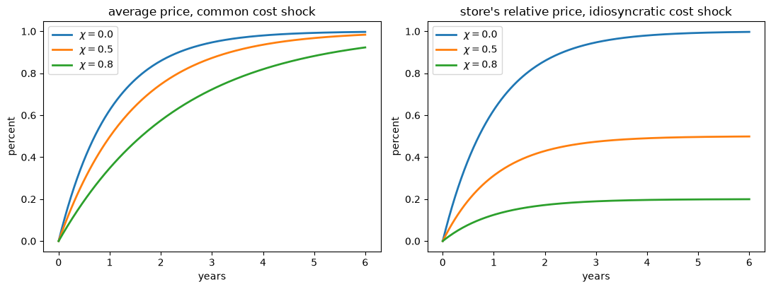
Fig. 127.1 Common and idiosyncratic cost pass-through#
A store passes an idiosyncratic cost increase through quickly but only partially, because its competitors’ prices do not move: in the long run it passes through \(1 - \chi\) of it.
The industry passes an aggregate cost increase through completely, but slowly, because each store waits for the others.
Let’s compare the half-lives.
for χ in (0.0, 0.5, 0.8):
    U_agg, U_dev = pricing_with_costs(χ, 0.0)
    λ_agg_f, λ_dev_f = U_agg[0, 0], U_dev[0, 0]
    print(f"χ = {χ}: store half-life {half_life(λ_dev_f):.2f} years, "
          f"industry half-life {half_life(λ_agg_f):.2f} years")
χ = 0.0: store half-life 0.71 years, industry half-life 0.71 years
χ = 0.5: store half-life 0.71 years, industry half-life 1.01 years
χ = 0.8: store half-life 0.71 years, industry half-life 1.62 years
With \(\chi = 0.8\) a store closes half of the gap to its new target in about 0.7 years, while the industry takes about 1.6 years.
The store’s half-life is the same for every \(\chi\), because a store’s deviation from the average is governed by its own curvature \(q\) alone.
So how fast stores respond to their own cost shocks reveals nothing about \(\chi\), which is the missing intercept of Linear Quadratic Mean Field Games in another guise.
How far they respond is a different matter: in the long run a store passes through \(1 - \chi\) of its own cost shock, because \(\chi\) also enters the store’s own return, through the weight on its cost.
When a model ties the own curvature \(Q\) to the interaction \(\Theta_X\) in this way, micro data can be informative after all; the result of the previous lecture is that, for given \(Q\), they are not.
Exercise 127.3 verifies Proposition 127.2 in this example and studies transitory cost shocks.
127.5. Coupling through higher moments#
So far agents have cared about the distribution of states only through its mean.
Alvarez and Argente [2026] also let payoffs depend on higher moments.
Take a scalar state and a scalar action, set \(\theta_{\mathcal A} = 0\), and write \(M_r(t) = \int x^r m(x,t) dx\) for the \(r\)-th moment of the cross-sectional distribution.
The period return is
the state follows \(dx = (b\alpha - ax)dt + \sigma dW\), and the benchmark of Linear Quadratic Mean Field Games is the case \(\bar r = 1\) and \(\theta_0 = 0\).
A natural notion of strategic complementarity is that a stochastically higher distribution raises the marginal return to \(x\), which here means that \(-\sum_r \theta_r x^r\) is nondecreasing in \(x\).
Our example below, with \(\theta_1\) and \(\theta_3\) negative and the other coefficients zero, satisfies it.
The value function is still quadratic, its curvature \(\bar\beta_2\) is still that of the single-agent problem, and the individual eigenvalue
is unchanged.
What changes is aggregation.
The Kolmogorov forward equation implies
so the moments obey a finite system, but a nonlinear one, because of the products \(\beta_1 M_{r-1}\).
When \(\sigma > 0\), \(\lambda_{\text{ind}} < 0\), and \(\theta_0 = -\sum_{r\ \mathrm{even}}\theta_r \bar M_r\), there is a steady state with \(\beta_1 = 0\) in which the invariant distribution is normal with mean zero and variance \(v = \sigma^2/(-2\lambda_{\text{ind}})\).
Its odd moments vanish and its even moments are \(\bar M_r = (r-1)!!\, v^{r/2}\); as \(\sigma \to 0\) it collapses to a point mass at zero, which we include below as a limiting case.
Linearizing the system around this steady state gives \(\dot y = \tilde{\mathcal H} y\) for \(y = (\hat\beta_1, \hat M_1, \ldots, \hat M_{\bar r})\), where hats denote deviations from the steady state.
Proposition 127.3
Let \(\bar r\) be even and define
The eigenvalues of \(\tilde{\mathcal H}\) are \(\tilde\lambda_r = r\lambda_{\text{ind}}\) for \(r = 2, \ldots, \bar r\), together with
If \(q + \bar\theta + \gamma a(a+\rho)/b^2 > 0\), the steady state is locally determinate, with one unstable and \(\bar r\) stable eigenvalues.
Three features stand out.
First, the interaction coefficients enter only through \(\bar\theta\), and only those on odd moments enter it, so \(\bar\theta\) plays exactly the role of \(\theta_X\) in the scalar formula of Linear Quadratic Mean Field Games.
Second, \(\bar\theta\) weights \(\theta_3, \theta_5, \ldots\) by even moments of the invariant distribution, which grow with \(\sigma^2\).
In the benchmark, the variance of idiosyncratic shocks never enters the Riccati equations, so it has no effect on aggregate dynamics; with higher moments, idiosyncratic risk affects aggregate persistence.
Third, coefficients on even moments do not affect the local eigenvalues, although they can affect transitional dynamics, as Exercise 127.4 shows.
Let’s build \(\tilde{\mathcal H}\) and check Proposition 127.3, using \(\bar r = 4\) and interactions through the first and third moments.
def moment_system(ρ, a, b, q, γ, σ, θ):
    """
    Linearized matrix for (β̂₁, M̂₁, ..., M̂_r̄) around the zero-mean steady
    state, with θ = (θ₁, ..., θ_r̄).  Also returns the steady-state moments
    M̄₀, ..., M̄_r̄ and the individual eigenvalue.
    """
    r_bar = len(θ)
    λ_ind = ρ/2 - np.sqrt((a + ρ/2)**2 + b**2*q/γ)
    v = σ**2/(-2*λ_ind)                       # invariant variance
    M_bar = np.zeros(r_bar + 1)
    M_bar[0] = 1.0
    for r in range(2, r_bar + 1, 2):
        M_bar[r] = (r - 1)*v*M_bar[r - 2]
    H_tilde = np.zeros((r_bar + 1, r_bar + 1))
    H_tilde[0, 0] = ρ - λ_ind
    H_tilde[0, 1:] = θ
    for r in range(1, r_bar + 1):
        H_tilde[r, 0] = r*M_bar[r - 1]*b**2/γ
        H_tilde[r, r] = r*λ_ind
        if r >= 3:                            # M̂₀ is identically zero
            H_tilde[r, r - 2] = r*(r - 1)*σ**2/2
    return H_tilde, M_bar, λ_ind

ρ_m, a_m, b_m, q_m, γ_m = 0.05, 0.3, 1.0, 1.0, 1.0
θ_m = np.array([-0.3, 0.0, -0.2, 0.0])       # complementarity through M₁ and M₃

for σ in (0.0, 0.5, 1.0):
    H_m, M_bar, λ_ind = moment_system(ρ_m, a_m, b_m, q_m, γ_m, σ, θ_m)
    θ_bar = θ_m[0] + 3*M_bar[2]*θ_m[2]
    root = np.sqrt((a_m + ρ_m/2)**2 + b_m**2*(q_m + θ_bar)/γ_m)
    predicted = np.r_[ρ_m/2 - root, ρ_m/2 + root, [r*λ_ind for r in range(2, 5)]]
    print(f"σ = {σ}: eigenvalues {np.sort(np.linalg.eigvals(H_m).real).round(4)}")
    print(f"        predicted   {np.sort(predicted).round(4)}")
σ = 0.0: eigenvalues [-4.1059 -3.0795 -2.053  -0.8726  0.9226]
        predicted   [-4.1059 -3.0795 -2.053  -0.8726  0.9226]
σ = 0.5: eigenvalues [-4.1059 -3.0795 -2.053  -0.8309  0.8809]
        predicted   [-4.1059 -3.0795 -2.053  -0.8309  0.8809]
σ = 1.0: eigenvalues [-4.1059 -3.0795 -2.053  -0.6915  0.7415]
        predicted   [-4.1059 -3.0795 -2.053  -0.6915  0.7415]
To trace the equilibrium path we keep the \(\bar r\) eigenvalues below \(\rho/2\), express \(\hat\beta_1\) as a linear function of the moment deviations on the stable subspace, and substitute.
That gives a law of motion for the moment deviations alone, so an initial condition specifies only those deviations, and \(\hat\beta_1(0)\) follows from the saddle path.
def moment_dynamics(H_tilde, ρ):
    "Law of motion of the moment deviations on the stable subspace of H_tilde."
    ev, V = np.linalg.eig(H_tilde)
    V_s = V[:, ev.real < ρ/2]
    s = np.real(V_s[0] @ np.linalg.inv(V_s[1:]))     # β̂₁ = s · M̂
    return H_tilde[1:, 1:] + np.outer(H_tilde[1:, 0], s)
As an initial condition we shift the invariant distribution to the right by \(\Delta\), which to first order raises \(M_1\) by \(\Delta\) and \(M_3\) by \(3v\Delta\) and leaves the even moments unchanged.
The next figure shows the path of the mean for several levels of idiosyncratic volatility.
t_m = np.linspace(0, 6, 200)
Δ = 0.1

fig, ax = plt.subplots(figsize=(8, 4.5))
for σ in (0.0, 0.6, 1.0, 1.3):
    H_m, M_bar, λ_ind = moment_system(ρ_m, a_m, b_m, q_m, γ_m, σ, θ_m)
    U_m = moment_dynamics(H_m, ρ_m)
    M_hat0 = np.array([Δ, 0.0, 3*M_bar[2]*Δ, 0.0])
    path = [(expm(U_m*t) @ M_hat0)[0] for t in t_m]
    θ_bar = θ_m[0] + 3*M_bar[2]*θ_m[2]
    λ_1 = ρ_m/2 - np.sqrt((a_m + ρ_m/2)**2 + b_m**2*(q_m + θ_bar)/γ_m)
    ax.plot(t_m, path, lw=2,
            label=f"$\\sigma = {σ}$, slowest half-life {half_life(λ_1):.2f}")
ax.set_xlabel('$t$')
ax.set_ylabel('cross-sectional mean $M_1(t)$')
ax.legend()
plt.tight_layout()
plt.show()
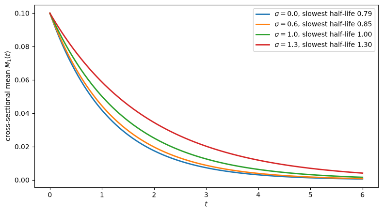
Fig. 127.2 Idiosyncratic risk and mean persistence#
Greater idiosyncratic volatility makes the mean more persistent here.
A larger variance puts more weight on the third moment, through which complementarity operates, so the effective interaction \(\bar\theta\) is stronger.
127.6. Exercises#
Exercise 127.1
This exercise continues the Hayashi example.
Choose \(\phi\) so that a firm that ignores the industry again closes half of a capital gap in three years under Hayashi costs, and recompute the industry’s half-life and the ratio of the two half-lives.
Holding \(\phi\) from part 1 and \(\varepsilon_s\) fixed, compute the aggregate eigenvalue in the limit of constant returns to scale, \(\nu \to 1\), where \(q + \theta_X \to 0\), once with no price effect and once with the calibrated supply elasticity. Explain why the answers differ from the limit \(\lambda \to -\delta\) that holds without Hayashi costs.
Solution
For part 1, the individual’s eigenvalue is \(\rho/2 - \sqrt{\rho^2/4 + \delta^2 q/\gamma}\), so a target \(\lambda\) requires \(\gamma = \delta^2 q/[(\rho/2 - \lambda)^2 - \rho^2/4]\).
λ_target = -np.log(2)/3
γ_H = δ_c**2*q_c/((ρ_c/2 - λ_target)**2 - ρ_c**2/4)

λ_ind_H = λ_cross(ρ_c, δ_c, δ_c, q_c + γ_H, γ_H, γ_H)
λ_agg_H = λ_cross(ρ_c, δ_c, δ_c, q_c + γ_H + θ_X_c, γ_H + θ_A_c, γ_H)

print(f"γ = {γ_H:.4f}, so φ = {γ_H/cap_scale(η_c, ν_c):.4f}")
print(f"individual half-life {half_life(λ_ind_H):.2f}, "
      f"industry half-life {half_life(λ_agg_H):.2f}, "
      f"ratio {half_life(λ_agg_H)/half_life(λ_ind_H):.2f}")
γ = 0.0384, so φ = 0.1097
individual half-life 3.00, industry half-life 5.42, ratio 1.81
Matching the three-year individual half-life requires a cheaper installation technology than before, \(\phi \approx 0.11\) instead of \(1/7\).
The industry’s half-life is then 5.4 years, so the gap between micro and macro adjustment widens: the ratio rises from 1.66 to 1.81.
For part 2, when \(q + \theta_X = 0\) the effective state curvature in Proposition 127.1 is \(\gamma\), and the industry’s effective return is
In the limit \(\nu \to 1\), the scale \(\delta\bar k^{1-\nu}\) that converts \(\phi\) and \(1/\varepsilon_s\) into \(\gamma\) and \(\theta_{\mathcal A}\) tends to \(\delta(\eta-1)/[\eta(\rho+\delta)]\).
Let’s compute the limit with and without a price effect.
φ_H = γ_H/cap_scale(η_c, ν_c)
scale_lim = cap_scale(η_c, 1.0)
γ_lim = φ_H*scale_lim
for inv_ε in (0.0, 1/ε_s_c):
    θ_A_lim = inv_ε*scale_lim
    λ_lim = λ_cross(ρ_c, δ_c, δ_c, γ_lim, γ_lim + θ_A_lim, γ_lim)
    print(f"1/ε_s = {inv_ε:.3f}: θ_A = {θ_A_lim:.4f}, λ = {λ_lim:.5f}")
1/ε_s = 0.000: θ_A = 0.0000, λ = 0.00000
1/ε_s = 0.257: θ_A = 0.1286, λ = -0.08054
With \(\theta_{\mathcal A} = 0\) the only cost is the cost of net investment, so any capital stock can be maintained for free and nothing pulls the industry back: the aggregate state has a unit root.
Without Hayashi costs, maintaining a capital stock above its steady state requires gross investment above \(\bar i\), which \(\psi(i)\) penalizes, so the industry lets depreciation do the work and \(\lambda \to -\delta\).
With \(\theta_{\mathcal A} > 0\) the price of investment goods penalizes gross investment away from \(\bar i\), which restores some mean reversion.
Exercise 127.2
This exercise shows why the restriction \(\Theta_{X\alpha} = \Theta_{x\mathcal A}\) matters, even with a single state.
Take \(\rho = 0.05\), \(a = 0.3\), \(b = q = \gamma = 1\), \(\theta_X = \theta_{\mathcal A} = 0\) and no own cross term, and use state_costate with \(C_1 = -\theta_{x\mathcal A}\) and \(C_2 = -\theta_{X\alpha}\).
Show that the trace of the state-costate matrix is \(\rho + b(\theta_{x\mathcal A} - \theta_{X\alpha})/(\gamma + \theta_{\mathcal A})\), so that its eigenvalues can be symmetric about \(\rho/2\) only when \(\theta_{X\alpha} = \theta_{x\mathcal A}\).
Compute the eigenvalues for \((\theta_{X\alpha}, \theta_{x\mathcal A})\) equal to \((0, 0)\), \((-2, -2)\), \((-1.5, -2.5)\) and \((-2.5, -1.5)\), and count how many have real parts below \(\rho/2\). What does each count imply about the number of equilibria?
Solution
For part 1, with \(g = \gamma + \theta_{\mathcal A}\) the diagonal elements of the matrix are \(\rho + a - b C_1/g\) and \(b C_2/g - a\).
Their sum is \(\rho + b(C_2 - C_1)/g = \rho + b(\theta_{x\mathcal A} - \theta_{X\alpha})/g\).
Eigenvalues symmetric about \(\rho/2\) must sum to \(\rho\), which requires \(\theta_{X\alpha} = \theta_{x\mathcal A}\).
For part 2, we compute the eigenvalues in each case.
ρ_e, a_e = 0.05, 0.3

print(f"{'(θ_Xα, θ_xA)':>14}{'eigenvalues':>34}{'trace':>8}{'below ρ/2':>11}")
for θ_Xα_e, θ_xA_e in ((0.0, 0.0), (-2.0, -2.0), (-1.5, -2.5), (-2.5, -1.5)):
    M_e = state_costate(a_e*one, one, one, one, ρ_e,
                        -θ_xA_e*one, -θ_Xα_e*one)
    ev = np.linalg.eigvals(M_e)
    print(f"{str((θ_Xα_e, θ_xA_e)):>14}{str(np.round(ev, 4)):>34}"
          f"{ev.real.sum():>8.3f}{np.sum(ev.real < ρ_e/2):>11}")
  (θ_Xα, θ_xA)                       eigenvalues   trace  below ρ/2
    (0.0, 0.0)                 [ 1.0765 -1.0265]   0.050          1
  (-2.0, -2.0)     [0.025+0.4409j 0.025-0.4409j]   0.050          0
  (-1.5, -2.5)                 [-0.7108 -0.2392]  -0.950          2
  (-2.5, -1.5)                   [0.2892 0.7608]   1.050          0
With no mixed interactions there is one eigenvalue on each side of \(\rho/2\) and a unique equilibrium.
At \((-2, -2)\) the restriction holds, but the sufficient condition \(q - \tilde C^2/g > 0\) of Proposition 127.1 fails, since \(1 - 4 < 0\).
The eigenvalues are then complex with real part exactly \(\rho/2\), so for \(X(0) \neq 0\) there is no admissible path and no equilibrium.
At \((-1.5, -2.5)\) both eigenvalues are below \(\rho/2\), so every initial costate \(w(0)\) generates an admissible path.
Each of these paths is an equilibrium.
Given aggregate paths that grow more slowly than \(e^{\rho t/2}\), the individual’s costate equation has a unique admissible solution, because its own root \(\rho - \lambda_{\text{ind}}\) exceeds \(\rho/2\), and the \(w\) on any path of the system is that solution.
So there is a continuum of equilibria for each initial distribution.
At \((-2.5, -1.5)\) both eigenvalues are above \(\rho/2\), and again no equilibrium exists for \(X(0) \neq 0\).
Exercise 127.3
This exercise works with the pricing example of Forcing processes and pass-through.
Take \(\chi = 0.8\) and \(a_{22} = 0.5\). Check that the eigenvalues of the aggregate closed-loop matrix are those of \(B_1\Gamma^{-1}B_1^\top P_{11} - A_{11}\) together with \(-a_{22}\), as Proposition 127.2 says. Check also that changing the \((2,2)\) elements of \(Q\) and \(\Theta_X\) leaves the first row of \(P\), and hence the pricing policy, unchanged.
With transitory cost shocks, \(a_{22} = 0.5\), plot the industry’s response to a common one percent cost increase for \(\chi \in \{0, 0.5, 0.8\}\). How do the size and timing of the peak response depend on \(\chi\)?
Solution
For part 1, we rebuild the example with the \((2,2)\) elements as arguments.
χ_e, a_22_e, ρ_f, q_f, γ_f = 0.8, 0.5, 0.04, 1.0, 1.0
A_f = np.array([[0.0, 0.0],
                [0.0, a_22_e]])
B_f = np.array([[1.0],
                [0.0]])
Γ_f = np.array([[γ_f]])

def P_forcing(q_22, θ_22):
    "Equilibrium P when the (2, 2) elements of Q and Θ_X are q_22 and θ_22."
    Q_f = q_f*np.array([[1.0, -(1 - χ_e)],
                        [-(1 - χ_e), 0.0]])
    Q_f[1, 1] = q_22
    Θ_f = np.array([[-q_f*χ_e, 0.0],
                    [0.0, θ_22]])
    return mfg_riccati(A_f, B_f, Q_f + Θ_f, Γ_f, ρ_f)

P_a, P_b = P_forcing(2.0, 0.0), P_forcing(7.0, 3.0)
λ_11 = P_a[0, 0]/γ_f          # B_1 Γ^{-1} B_1' P_11 - A_11
ev_cl = np.sort(np.linalg.eigvals(closed_loop(A_f, B_f, Γ_f, P_a)).real)
print("closed-loop eigenvalues:   ", ev_cl.round(5))
print("controlled block and -a_22:", np.sort([λ_11, -a_22_e]).round(5))
print("first row of P unchanged:", np.allclose(P_a[0], P_b[0]))
closed-loop eigenvalues:    [-0.5     -0.42766]
controlled block and -a_22: [-0.5     -0.42766]
first row of P unchanged: True
For part 2, we plot the response of the average price.
t_e = np.linspace(0, 8, 400)
fig, ax = plt.subplots(figsize=(8, 4.5))
for χ in (0.0, 0.5, 0.8):
    U_agg, _ = pricing_with_costs(χ, 0.5)
    agg = np.array([(expm(U_agg*t) @ np.array([0.0, 1.0]))[0] for t in t_e])
    k = agg.argmax()
    ax.plot(t_e, agg, lw=2, label=f"$\\chi = {χ}$")
    print(f"χ = {χ}: peak {agg[k]:.3f} percent after {t_e[k]:.2f} years")
ax.set_xlabel('years')
ax.set_ylabel('average price, percent')
ax.legend()
plt.tight_layout()
plt.show()
χ = 0.0: peak 0.333 percent after 1.40 years
χ = 0.5: peak 0.253 percent after 1.70 years
χ = 0.8: peak 0.164 percent after 2.17 years
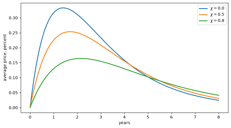
Stronger complementarity makes the peak response smaller and later.
Each store raises its price more slowly because the others do, so by the time the industry’s price has risen much, the cost shock has already started to fade.
Exercise 127.4
This exercise shows how an interaction through an even moment affects transitional dynamics without changing the local eigenvalues.
Take \(\bar r = 2\), \(\theta_1 = -0.3\), \(\sigma = 1\) and the other parameters of the moment example in Coupling through higher moments.
Verify that \(\theta_2\) changes none of the eigenvalues of \(\tilde{\mathcal H}\).
Suppose the cross-sectional variance rises by 0.1 while the mean stays at zero. Trace the path of the mean for \(\theta_2 \in \{-0.5, 0, 0.5\}\) and explain what you see.
Alvarez and Argente [2026] show that along the saddle path \(\dot{\hat M}_1 = \tilde\lambda_1\hat M_1 + \zeta\hat M_2\) with \(\zeta = b^2\theta_2/[\gamma(\tilde\lambda_1 + 2\lambda_{\text{ind}} - \rho)]\). Check this formula.
Solution
For part 1, we compute the eigenvalues for each \(\theta_2\).
θ_1 = -0.3
for θ_2 in (-0.5, 0.0, 0.5):
    H_2, _, _ = moment_system(ρ_m, a_m, b_m, q_m, γ_m, 1.0, np.array([θ_1, θ_2]))
    print(f"θ_2 = {θ_2:>4}: eigenvalues {np.sort(np.linalg.eigvals(H_2).real).round(5)}")
θ_2 = -0.5: eigenvalues [-2.05297 -0.87257  0.92257]
θ_2 =  0.0: eigenvalues [-2.05297 -0.87257  0.92257]
θ_2 =  0.5: eigenvalues [-2.05297 -0.87257  0.92257]
They do not move.
At the zero-mean steady state the second moment evolves on its own, \(\dot{\hat M}_2 = 2\lambda_{\text{ind}}\hat M_2\), because the term \(2(b^2/\gamma)\beta_1 M_1\) in its law of motion vanishes to first order.
For part 2, we start from \(\hat M_1 = 0\) and \(\hat M_2 = 0.1\).
t_e = np.linspace(0, 4, 200)
fig, ax = plt.subplots(figsize=(8, 4.5))
for θ_2 in (-0.5, 0.0, 0.5):
    H_2, _, _ = moment_system(ρ_m, a_m, b_m, q_m, γ_m, 1.0, np.array([θ_1, θ_2]))
    U_2 = moment_dynamics(H_2, ρ_m)
    path = [(expm(U_2*t) @ np.array([0.0, 0.1]))[0] for t in t_e]
    ax.plot(t_e, path, lw=2, label=f"$\\theta_2 = {θ_2}$")
ax.set_xlabel('$t$')
ax.set_ylabel('cross-sectional mean $M_1(t)$')
ax.legend()
plt.tight_layout()
plt.show()
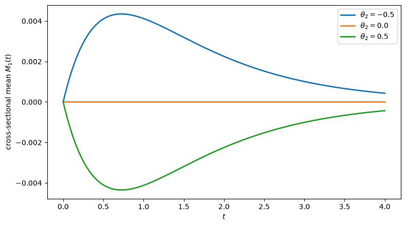
With \(\theta_2 > 0\), a higher second moment lowers everybody’s marginal return to \(x\) through the term \(-\theta_2 M_2 x\), so agents lower \(x\) while the variance is high, and the mean dips before returning as the variance returns to its invariant level.
With \(\theta_2 < 0\) the mean rises instead, and with \(\theta_2 = 0\) it does not move at all.
So a shock to dispersion moves the average, even though the eigenvalues that govern local persistence are unchanged.
For part 3, we compare the coefficients of the saddle-path law of motion with the formula.
for θ_2 in (-0.5, 0.5):
    H_2, _, λ_ind_2 = moment_system(ρ_m, a_m, b_m, q_m, γ_m, 1.0, np.array([θ_1, θ_2]))
    U_2 = moment_dynamics(H_2, ρ_m)
    λ_1 = ρ_m/2 - np.sqrt((a_m + ρ_m/2)**2 + b_m**2*(q_m + θ_1)/γ_m)
    ζ = b_m**2*θ_2/(γ_m*(λ_1 + 2*λ_ind_2 - ρ_m))
    print(f"θ_2 = {θ_2}: coefficients ({U_2[0, 0]:.5f}, {U_2[0, 1]:.5f}), "
          f"formula ({λ_1:.5f}, {ζ:.5f})")
θ_2 = -0.5: coefficients (-0.87257, 0.16804), formula (-0.87257, 0.16804)
θ_2 = 0.5: coefficients (-0.87257, -0.16804), formula (-0.87257, -0.16804)
127.7. Further reading#
Alvarez and Argente [2026] develop the cross terms and the forcing processes in the appendices of their paper, and the coupling through higher moments in its main text.
The Hayashi and pass-through examples, and the one-state analysis of the mixed interactions in Exercise 127.2, are our own illustrations of their results.