31. Incentives for Information Transfer#
31.1. Overview#
In many organizations the person who gathers information is not the person who acts on it.
A stockbroker studies a firm and a client decides whether to buy its stock.
A physician examines a patient and the patient chooses a treatment.
A division manager knows local conditions and headquarters allocates capital among divisions.
When the informant and the decision maker want different things, the informant may misreport what he has seen.
Green [1982] studies a decision maker, the planner, who must elicit an observation from an agent whose preferences over the planner’s actions differ from hers.
The planner moves first and commits to an action plan, a rule that maps each possible report into a probability distribution over actions.
The agent then observes a signal drawn from a statistical experiment, forms a posterior, and sends whichever report the action plan rewards most.
Green obtains the following results.
The planner loses nothing by confining herself to plans under which the agent prefers to report truthfully, so the planner’s problem is a single linear program.
With two actions, the planner can do no better than either ignoring the agent or letting him have his way; with two actions and two signals, she either attains her first-best outcome or gains nothing from the agent.
With more than two actions, the optimal plan can randomize, and it can put positive probability on an action that the planner would never take if she saw the signal herself.
Truthful reporting does not mean that all information is used: the optimal plan can pool some signals while distinguishing others.
Giving the agent a more informative experiment, in the sense of Blackwell’s Theorem on Comparing Experiments, can lower the planner’s expected utility.
That cannot happen when both experiments have only two signals.
Results 5 and 6 connect Green’s model to Blackwell’s theorem.
A decision maker who sees a signal herself never prefers a less informative experiment.
A planner who must elicit the signal from someone else sometimes does, because a sharper signal can open a conflict of interest that a coarser signal hides.
To compare experiments, Green uses a characterization of Blackwell’s order in terms of posterior probabilities that is due to Marschak and Miyasawa [1968].
We will see that their characterization turns the question “is one experiment a garbling of another?” into a transport problem of the kind studied in Optimal Transport, with one additional set of constraints.
The paper was published with comments by Postlewaite [1982] and Riley [1982].
The exercises work through their examples and through a comparison of information conditions from Marschak and Miyasawa [1968].
The lecture proceeds as follows.
We set up a statistical decision problem in Green’s notation.
We add an agent, state Green’s revelation principle, and solve the planner’s linear program.
We study economies with two actions, and Green’s examples of randomization and of pooled signals.
We use the Marschak–Miyasawa characterization to compare experiments, show how better information can hurt the planner, and prove that it cannot when both experiments have two signals.
We report what the discussants added, and relate Green’s model to other lectures and to later work on communication and delegation.
We begin with some imports.
import numpy as np
import matplotlib.pyplot as plt
from scipy.optimize import linprog
from itertools import product

np.set_printoptions(precision=4, suppress=True)
31.2. A statistical decision problem#
31.2.1. States, signals, and actions#
There are \(M\) states of nature \(\theta_1, \ldots, \theta_M\) with prior probabilities \(\pi = (\pi_1, \ldots, \pi_M)\).
Before acting, someone observes one of \(N\) signals \(y_1, \ldots, y_N\).
The \(M \times N\) likelihood matrix \(\Lambda = [\lambda_{mn}]\), which we also call an experiment, has entries
so each row of \(\Lambda\) is a probability distribution over signals.
The signal probabilities and the posterior probabilities of the states are
We collect the posteriors in the \(M \times N\) matrix \(P = [p_{mn}]\), whose \(n\)th column \(p_n\) is the posterior after signal \(y_n\).
There are \(K\) actions \(a_1, \ldots, a_K\).
A \(K \times M\) utility matrix \(U = [u_{km}]\) gives the utility \(u_{km}\) of action \(a_k\) in state \(\theta_m\).
The \((k, n)\) entry of the \(K \times N\) matrix \(UP\) is the expected utility of action \(a_k\) after signal \(y_n\).
A decision maker who observes the signal herself takes, in each column of \(UP\), the action with the largest entry.
We call this rule her first-best plan and her expected utility
her first-best value.
Without a signal she takes the action that maximizes \((U\pi)_k\), and her expected utility is \(v_0 = \max_k (U\pi)_k\).
The following functions compute posteriors and the two benchmark values \(v(\Lambda)\) and \(v_0\).
def posteriors(Λ, π):
    """Signal probabilities q and the M x N matrix P of posteriors."""
    joint = π[:, None] * Λ
    q = joint.sum(axis=0)
    if np.any(q <= 0):
        raise ValueError("every signal must have positive probability")
    return q, joint / q


def bayes_value(U, Λ, π):
    """Expected utility of a decision maker who sees the signal herself."""
    q, P = posteriors(Λ, π)
    return q @ (U @ P).max(axis=0)


def no_info_value(U, π):
    """Expected utility of the best action taken without a signal."""
    return (U @ π).max()
31.3. A planner and an agent#
31.3.1. Action plans and reports#
Now suppose that the signal is observed not by the decision maker but by an agent.
From here on we call the decision maker the planner.
The agent cares about the planner’s action and the state, and his utilities are the entries of a \(K \times M\) matrix \(W = [w_{km}]\).
Green writes \(U'\) for the agent’s matrix; we use \(W\) and keep primes for alternative experiments.
The planner and the agent share the prior \(\pi\), and both know \(\Lambda\), \(U\), and \(W\).
Events unfold as follows.
The planner announces an action plan, an \(N \times K\) Markov matrix \(Z = [z_{nk}]\), that is, a nonnegative matrix whose rows sum to one; \(z_{nk}\) is the probability that she takes action \(a_k\) when the agent reports \(y_n\).
The agent observes a signal \(y_n\), and his posterior is \(p_n\).
The agent reports some signal \(y_r\), which need not equal \(y_n\).
The planner draws an action from row \(r\) of \(Z\).
Let
The \((r, n)\) entry of the \(N \times N\) matrix \(V\) is the agent’s expected utility when he has seen \(y_n\) and reports \(y_r\).
So the agent’s best reports are the largest entries in each column of \(V\).
The planner is committed: once the agent has spoken, she carries out the announced randomization even if, given the report, another action looks better to her.
Green stresses that this includes the draw itself.
After report \(y_r\) she must take whatever action the lottery in row \(r\) produces; she cannot substitute her favorite among the actions that the row allows and claim that the lottery chose it.
In this sense the planner is a Stackelberg leader, as in Stackelberg plans.
Commitment lets her make threats, such as the dominated action in Green’s first example below, that she would not carry out if she could reoptimize after hearing the report.
The value of being able to commit is also the theme of The Credibility Problem, which studies the Kydland–Prescott model of monetary policy.
Without commitment the planner would take her best action given her beliefs after each report, and we would be in the cheap-talk world of Crawford and Sobel [1982].
31.3.2. The revelation principle#
A plan \(Z\) induces a response rule \(\rho\): after observing \(y_n\), the agent reports \(y_{\rho(n)}\).
Following Green, a response rule is a deterministic map from observations to reports.
Green’s first result says that the planner can restrict herself to plans whose response rule is the identity.
Theorem 31.1 (Revelation principle (Green’s Theorem 1))
The highest expected utility that the planner can attain over all action plans, when the agent responds to each plan with a response rule that is optimal for him, equals the value of the linear program
subject to \(z_{nk} \geq 0\), \(\sum_k z_{nk} = 1\) for every \(n\), and the truth-telling constraints \(V_{nn} \geq V_{rn}\) for all \(n\) and \(r\), that is,
The theorem is a version of the revelation principle of mechanism design; Myerson [1979] is the reference that Green cites as closest to his analysis.
Here is the argument.
Suppose that plan \(Z\) induces the response rule \(\rho\).
Build a new plan \(\hat Z\) whose \(n\)th row is row \(\rho(n)\) of \(Z\).
The rows of \(\hat Z\) are among the rows of \(Z\), so the agent has no new options.
After observing \(y_n\) he chose row \(\rho(n)\) of \(Z\) before, so he is willing to choose row \(n\) of \(\hat Z\), which is the same lottery.
Under \(\hat Z\) and truthful reports, the planner’s action after each observation has the same distribution as under \(Z\) and the original reports, so her expected utility is the same.
Green writes the truth-telling constraints as weak inequalities, so an indifferent agent is assumed to report truthfully.
We write \(\hat v(\Lambda)\) for the value of the linear program.
A plan that ignores the agent’s report satisfies the truth-telling constraints, and no plan can do better than a planner who sees the signal herself, so
Riley [1982] remarks that, appropriately interpreted, the revelation principle is essentially definitional: the agent simply picks one lottery from the menu formed by the rows of \(Z\).
That reading makes Green’s planner a designer of a menu from which a better-informed subordinate chooses, a theme of the work on delegation discussed at the end of this lecture.
Truth-telling does not mean that all information gets through: if two rows of \(Z\) are equal, the planner treats the two corresponding signals identically, as Green’s second example will show.
31.3.3. Solving the linear program#
We stack the entries of \(Z\) row by row into a vector of length \(NK\) and pass the problem to SciPy’s linprog.
The constraints that each row of \(Z\) sums to one then take the Kronecker-product form np.kron(np.eye(N), np.ones(K)).
Optimal Transport stacks columns instead, so there the same form encodes column sums.
Because linprog minimizes, we pass the negative of the planner’s objective.
def solve_planner(U, W, Λ, π, ties=None):
    """
    Solve the planner's linear program of Green's revelation principle.

    U, W : K x M utility matrices of the planner and the agent
    Λ    : M x N likelihood matrix
    π    : prior over the M states
    ties : None, "agent_best", or "agent_worst"; when the planner has
           several optimal plans, return the one that the agent likes
           best or least, instead of the one the solver happens to find

    Returns the N x K action plan Z, the planner's optimal expected
    utility, and the agent's expected utility under Z when he reports
    truthfully.
    """
    q, P = posteriors(Λ, π)
    K, N = U.shape[0], Λ.shape[1]
    UP, WP = U @ P, W @ P

    # Entry n * K + k of the decision vector is z_{nk}
    planner_obj = (UP * q).T.ravel()
    agent_obj = (WP * q).T.ravel()

    # For every true signal n and every false report r,
    # sum_k (z_{rk} - z_{nk}) (WP)_{kn} <= 0
    rows = []
    for n in range(N):
        for r in range(N):
            if r != n:
                row = np.zeros((N, K))
                row[r] += WP[:, n]
                row[n] -= WP[:, n]
                rows.append(row.ravel())
    A_ub = np.array(rows).reshape(-1, N * K)
    b_ub = np.zeros(len(A_ub))

    # Each row of Z sums to one
    A_eq = np.kron(np.eye(N), np.ones(K))
    b_eq = np.ones(N)

    def solve(c, A_ub, b_ub):
        # HiGHS's presolve step occasionally misreports these small
        # problems as infeasible, so we switch it off
        res = linprog(c, A_ub=A_ub, b_ub=b_ub, A_eq=A_eq, b_eq=b_eq,
                      bounds=(0, None), method="highs",
                      options={"presolve": False})
        if res.status != 0:
            raise RuntimeError(res.message)
        return res.x

    x = solve(-planner_obj, A_ub, b_ub)
    planner = planner_obj @ x
    if ties is not None:
        # Among plans worth the planner's optimum up to a small tolerance,
        # make the agent as well off (or as badly off) as possible; the
        # plan returned is then optimal for the planner up to that tolerance
        sign = {"agent_best": -1, "agent_worst": 1}[ties]
        tol = 1e-8 * max(1, abs(planner))
        x = solve(sign * agent_obj, np.vstack([A_ub, -planner_obj]),
                  np.append(b_ub, -planner + tol))
    # Remove round-off below zero, and turn -0.0 into 0.0
    Z = np.maximum(x, 0.0).reshape(N, K) + 0.0
    return Z, planner, agent_obj @ x
When the planner has several optimal plans, the agent’s expected utility can differ across them.
With ties=None, solve_planner reports the agent’s utility at whichever optimal plan the solver finds.
With ties="agent_best" or ties="agent_worst", it solves a second linear program that holds the planner at her optimal value and makes the agent as well off, or as badly off, as possible.
31.4. Economies with two actions#
With two actions the planner’s problem becomes simple, as Green’s next two results show.
Green proves the first one for two states, but the argument below works for any number of states and signals.
Theorem 31.2 (Two actions (Green’s Theorem 3))
If \(K = 2\), the planner has an optimal plan that either ignores the agent’s report or takes, after every signal, the action that the agent would choose if he were the decision maker.
In the second case the planner implements the agent’s first-best plan, not her own.
With two actions, a row of \(Z\) is determined by \(z_{n1}\), the probability of \(a_1\) after report \(y_n\), which in this section we write simply as \(z_n\).
After observing \(y_n\), the agent values a report \(y_r\) at
so whatever signal he has seen, the agent ranks the rows of \(Z\) by \(z_r\) alone.
He reports the signal with the largest \(z_r\) when he prefers \(a_1\) at his posterior, and the one with the smallest \(z_r\) when he prefers \(a_2\).
Truth-telling therefore forces \(z_n\) to take one common value \(z_{\rm hi}\) on the signals after which the agent prefers \(a_1\), and another common value \(z_{\rm lo} \leq z_{\rm hi}\) on the others, at least when the agent is never exactly indifferent.
If the agent prefers the same action after every signal, all the \(z_n\) are equal and the plan ignores the report.
Otherwise the planner’s expected utility is linear in \((z_{\rm lo}, z_{\rm hi})\) on the triangle \(0 \leq z_{\rm lo} \leq z_{\rm hi} \leq 1\), so it reaches its maximum at a vertex.
Two vertices, \((0, 0)\) and \((1, 1)\), ignore the report, and the third, \((0, 1)\), gives the agent his preferred action after every signal.
So \(\hat v(\Lambda) = \max\{v_0, v_A(\Lambda)\}\), where \(v_A(\Lambda)\) is the planner’s expected utility when she takes the agent’s preferred action after every signal; if the agent is sometimes indifferent, his ties should be broken in the planner’s favor.
The theorem says that an optimal plan takes one of the two forms.
When the planner’s objective is constant along an edge of the triangle, the plans in between are optimal too, and they can give the agent different payoffs.
Green states that the solution “must be” one of the two types, but his own third example, studied below, has optimal plans of neither type.
With two signals as well as two actions, the planner gets all or nothing.
Corollary 31.1 (Two actions and two signals (Green’s Theorem 2))
If \(K = N = 2\), then either \(\hat v(\Lambda) = v(\Lambda)\), so that the planner attains her first best, or \(\hat v(\Lambda) = v_0\), so that the agent’s information is worthless to her.
If the two players’ first-best plans coincide, the planner announces hers, the agent reports truthfully, and \(\hat v(\Lambda) = v(\Lambda)\).
Suppose instead that the plans differ, and, to keep the argument short, that neither player is ever indifferent.
By Theorem 31.2, \(\hat v(\Lambda) = \max\{v_0, v_A(\Lambda)\}\), so it suffices to show that \(v_A(\Lambda) \leq v_0\).
If the agent prefers the same action after both signals, his first-best plan takes a single action, which is worth at most \(v_0\) to the planner.
If the agent’s preferred action differs across the signals and the planner’s does not, then \(v_A(\Lambda) \leq v(\Lambda) = v_0\).
If both players’ preferred actions differ across the signals, then they are reversed, so the agent’s first-best plan gives the planner the action she likes less after both signals, and either action taken after both signals does better.
In each case \(\hat v(\Lambda) = v_0\).
This proves the corollary and sharpens it: with two actions and two signals, unless the players have a first-best plan in common, the agent’s information is worthless to the planner.
To check both results numerically, we draw random economies in which the players’ first-best plans differ after at least one signal, since otherwise the planner trivially attains her first best.
The two players’ utilities are positively correlated, so that they agree often but not always.
def random_economy(M, K, N, rng, corr=0.8):
    """Random prior, likelihood matrix, and utilities with correlation corr."""
    π = rng.dirichlet(np.ones(M))
    Λ = rng.dirichlet(np.ones(N), size=M)
    U = rng.normal(size=(K, M))
    W = corr * U + np.sqrt(1 - corr**2) * rng.normal(size=(K, M))
    return U, W, Λ, π


def plans_differ(U, W, Λ, π):
    """True if the players' preferred actions differ after some signal."""
    _, P = posteriors(Λ, π)
    return np.any((U @ P).argmax(axis=0) != (W @ P).argmax(axis=0))


def agent_plan_value(U, W, Λ, π):
    """Planner's expected utility when the agent's preferred action is taken."""
    q, P = posteriors(Λ, π)
    k = (W @ P).argmax(axis=0)
    return q @ (U @ P)[k, np.arange(len(q))]


rng = np.random.default_rng(1234)

gaps, agent_wins = [], 0
while len(gaps) < 500:
    M, N = rng.integers(2, 5), rng.integers(2, 6)
    U, W, Λ, π = random_economy(M, 2, N, rng)
    if not plans_differ(U, W, Λ, π):
        continue
    v_hat = solve_planner(U, W, Λ, π)[1]
    v_0, v_A = no_info_value(U, π), agent_plan_value(U, W, Λ, π)
    gaps.append(abs(v_hat - max(v_0, v_A)))
    agent_wins += v_A > v_0 + 1e-10
print(f"K = 2: largest gap {max(gaps):.1e}; letting the agent have his way "
      f"beats ignoring him in {agent_wins} of {len(gaps)} draws")

gaps = []
while len(gaps) < 500:
    U, W, Λ, π = random_economy(rng.integers(2, 5), 2, 2, rng)
    if not plans_differ(U, W, Λ, π):
        continue
    gaps.append(abs(solve_planner(U, W, Λ, π)[1] - no_info_value(U, π)))
print(f"K = N = 2: largest gap between v_hat and v_0 {max(gaps):.1e}")
K = 2: largest gap 1.5e-15; letting the agent have his way beats ignoring him in 48 of 500 draws
K = N = 2: largest gap between v_hat and v_0 8.9e-16
In every draw, the value of the linear program equals the value \(\max\{v_0, v_A(\Lambda)\}\) that the theorem predicts, up to rounding error.
With two actions and two signals, it always equals \(v_0\), as the sharpened version of Corollary 31.1 says.
With more signals, letting the agent have his way sometimes beats ignoring him, but in most draws it does not.
31.5. Dominated actions as threats#
With two actions a lottery is just a probability of \(a_1\), so the agent’s ranking of lotteries is fixed by which action he prefers, and the planner can do no better than ignoring him or deferring to him.
With three actions, the agent’s ranking of lotteries can change with his posterior even when his ranking of the actions themselves does not, and that lets the planner do better than both.
Green’s first example has two states, two signals, and three actions.
The prior is uniform and
The posterior probability of \(\theta_1\) is \(3/4\) after \(y_1\) and \(1/4\) after \(y_2\).
If the planner saw the signal, she would take \(a_2\) after \(y_1\) and \(a_1\) after \(y_2\).
The agent prefers \(a_2\) after either signal, so if the planner announced her first-best plan, an agent who saw \(y_2\) would report \(y_1\).
Action \(a_3\) yields the planner \(-1\) in both states, while \(a_2\) yields \(0\), so a planner who saw the signal would never take \(a_3\).
Let’s solve the planner’s linear program.
π_ex1 = np.array([1/2, 1/2])
Λ_ex1 = np.array([[3/4, 1/4],
                  [1/4, 3/4]])
U_ex1 = np.array([[-2.0, 3.0],
                  [0.0, 0.0],
                  [-1.0, -1.0]])
W_ex1 = np.array([[0.0, -1.0],
                  [2.0, 0.0],
                  [0.0, -4.0]])

Z_ex1, v_ex1, _ = solve_planner(U_ex1, W_ex1, Λ_ex1, π_ex1)
print("optimal plan Z =\n", Z_ex1)
print(f"planner: {v_ex1:.4f}"
      f"   first best: {bayes_value(U_ex1, Λ_ex1, π_ex1):.4f}"
      f"   no information: {no_info_value(U_ex1, π_ex1):.4f}")
optimal plan Z =
 [[0.     0.6429 0.3571]
 [1.     0.     0.    ]]
planner: 0.6964   first best: 0.8750   no information: 0.5000
The optimal plan takes \(a_1\) after report \(y_2\); after report \(y_1\) it takes \(a_2\) with probability \(9/14\) and the dominated action \(a_3\) with probability \(5/14\).
The planner’s expected utility is \(\hat v(\Lambda) = 39/56 \approx 0.696\), between the \(v_0 = 0.5\) she gets by ignoring the agent and the \(v(\Lambda) = 0.875\) she would get if she saw the signal herself.
Green reports \(0.696\) and the probabilities \(0.643\) and \(0.357\).
Why does a dominated action help?
The plan must deter an agent who has seen \(y_2\) from reporting \(y_1\), so it attaches to report \(y_1\) an action that this agent dislikes.
Measure each candidate threat against \(a_2\), the action the planner would like to take after \(y_1\).
At the truthful posterior \(3/4\), action \(a_3\) costs the planner \(1\), while at the posterior \(1/4\) of an agent who lies, it costs him \(1/2 - (-3) = 7/2\).
Action \(a_1\) would cost the planner only \(3/4\), but it would cost the lying agent only \(1/2 - (-3/4) = 5/4\).
So \(a_3\) imposes \(7/2\) on a liar per unit of cost to the planner, against \(5/3\) for \(a_1\).
It is the cheaper threat because it hurts the agent most in state \(\theta_2\), which an agent who has seen \(y_2\) thinks likely.
An agent who has seen \(y_2\) gets \(-3/4\) from telling the truth, so the threat must lower what he gets from claiming \(y_1\) by \(1/2 - (-3/4) = 5/4\).
With \(a_3\) that takes probability \((5/4)/(7/2) = 5/14\), which leaves him exactly indifferent between telling the truth and lying; with \(a_1\) it would take probability one.
Randomization and the dominated action are needed together.
Deterministic plans fail: after either signal the agent ranks the actions in the same order, \(a_2\), then \(a_1\), then \(a_3\), so any plan that takes different actions after the two reports tempts an agent who has seen one of the signals to lie, and the best plan that takes the same action after both reports is worth \(v_0\).
Without \(a_3\) there are only two actions, and the agent prefers \(a_2\) at both posteriors, so by the argument behind Theorem 31.2 truth-telling forces the plan to treat the two reports alike; the best such plan takes \(a_1\) after both reports and is worth only \(v_0\).
v_no_threat = solve_planner(U_ex1[:2], W_ex1[:2], Λ_ex1, π_ex1)[1]
print(f"planner's value without a_3: {v_no_threat:.4f}")
planner's value without a_3: 0.5000
The figure below plots each player’s expected utility from each action against the posterior probability of \(\theta_1\).
The dashed line is the expected utility of the lottery that the plan attaches to report \(y_1\), and the dotted vertical lines mark the two posteriors.
p_grid = np.linspace(0, 1, 200)
lottery = Z_ex1[0]

fig, axes = plt.subplots(1, 2, figsize=(10, 4))
for ax, mat, who, loc in zip(axes, (U_ex1, W_ex1), ("planner", "agent"),
                             ("upper right", "lower right")):
    for k in range(3):
        ax.plot(p_grid, mat[k, 0] * p_grid + mat[k, 1] * (1 - p_grid),
                lw=2, label=f"$a_{k+1}$")
    mix = lottery @ mat
    ax.plot(p_grid, mix[0] * p_grid + mix[1] * (1 - p_grid),
            "k--", lw=2, label="plan after report $y_1$")
    for p_n in (1/4, 3/4):
        ax.axvline(p_n, color="0.6", lw=1, ls=":")
    ax.set_xlabel(r"posterior probability of $\theta_1$")
    ax.set_ylabel(f"expected utility of the {who}")
    ax.legend(loc=loc)

plt.tight_layout()
plt.show()
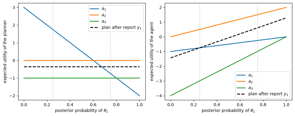
Fig. 31.1 Expected utilities in Green’s first example#
In the right panel the dashed line meets the agent’s line for \(a_1\) exactly at the posterior \(1/4\), where the agent who has seen \(y_2\) is indifferent.
At the posterior \(3/4\) the dashed line lies far above the line for \(a_1\), so an agent who has seen \(y_1\) strictly prefers to report it.
In the left panel the dashed line lies below the line for \(a_2\).
The gap at the posterior \(3/4\), \(5/14\), is the planner’s loss after report \(y_1\).
Since \(y_1\) has probability \(1/2\), her expected cost of eliciting the truth is \(5/28 = v(\Lambda) - \hat v(\Lambda)\).
31.6. Truthful but coarse reports#
Green’s second example shows a different way in which incentives can cost the planner information.
There are three signals with equal probabilities, and Green specifies the expected-utility matrices directly:
We can represent these by three equally likely states, a uniform prior, and a perfectly informative experiment \(\Lambda = I\), for which \(P = I\).
π_ex2 = np.full(3, 1/3)
Λ_ex2 = np.eye(3)
U_ex2 = np.array([[5.0, -1.0, -1.0],
                  [0.0, 0.0, 0.0],
                  [0.0, 0.0, 0.0]])
W_ex2 = np.array([[1.0, 1.5, 0.0],
                  [0.0, 1.0, 0.0],
                  [0.0, 0.0, 1.0]])

Z_ex2, v_ex2, _ = solve_planner(U_ex2, W_ex2, Λ_ex2, π_ex2)
print("optimal plan Z =\n", Z_ex2)
print(f"planner: {v_ex2:.4f}"
      f"   first best: {bayes_value(U_ex2, Λ_ex2, π_ex2):.4f}"
      f"   no information: {no_info_value(U_ex2, π_ex2):.4f}")
optimal plan Z =
 [[1. 0. 0.]
 [1. 0. 0.]
 [0. 1. 0.]]
planner: 1.3333   first best: 1.6667   no information: 1.0000
The planner wants \(a_1\) only after \(y_1\), but an agent who has seen \(y_2\) also likes \(a_1\), which is worth \(3/2\) to him, more than either other action.
Suppose that after report \(y_1\) the plan takes \(a_1\) with probability \(\alpha\) and fills the rest of the row with \(a_3\), the action that an agent who has seen \(y_2\) likes least, and that after report \(y_2\) it takes \(a_1\) with probability \(\beta\) and \(a_2\) otherwise.
An agent who has seen \(y_2\) gets \(1 + \beta/2\) from telling the truth and \(3\alpha/2\) from claiming \(y_1\), so truth requires \(\beta \geq 3\alpha - 2\).
So the best plan that never takes \(a_1\) after report \(y_2\) takes it with probability \(2/3\) after report \(y_1\), which is worth \(10/9\) to the planner.
Beyond \(\alpha = 2/3\), each unit of probability on \(a_1\) after report \(y_1\) gains the planner \(5\) but forces three units on \(a_1\) after report \(y_2\), each costing her \(1\), so she raises \(\alpha\) all the way to \(1\).
The optimal plan therefore gives the same lottery, \(a_1\) for sure, after reports \(y_1\) and \(y_2\), and the linear program confirms that no plan outside this family does better.
The agent reports truthfully, but the planner treats the first two signals identically and earns \(4/3\), which lies between the \(1\) of ignoring the agent and the \(5/3\) of the first best.
The third row of \(Z\) is not pinned down: after report \(y_3\) the planner is indifferent between \(a_2\) and \(a_3\), and the agent’s expected utility depends on which she takes.
for ties in ("agent_worst", "agent_best"):
    agent = solve_planner(U_ex2, W_ex2, Λ_ex2, π_ex2, ties=ties)[2]
    print(f"{ties}: agent {agent:.4f}")
agent_worst: agent 0.8333
agent_best: agent 1.1667
Across the planner’s optimal plans, the agent’s expected utility ranges from \(5/6\) to \(7/6\).
31.7. Comparing experiments#
31.7.1. Blackwell’s order through posteriors#
To ask whether the planner wants her agent to be better informed, Green needs a way to rank experiments.
Let \(\Lambda'\) be another experiment, with \(N'\) signals \(y'_1, \ldots, y'_{N'}\), and let primes mark everything computed from it, such as \(q'\) and \(P'\).
By Theorem 30.1, \(v(\Lambda) \geq v(\Lambda')\) for every utility matrix \(U\) and every prior \(\pi\) if and only if \(\Lambda' = \Lambda B\) for some \(N \times N'\) Markov matrix \(B\).
When that holds, \(\Lambda\) is (weakly) more informative than \(\Lambda'\), and \(\Lambda'\) is a garbling of \(\Lambda\).
Note
In Blackwell’s Theorem on Comparing Experiments, an experiment is written \(\mu\) rather than \(\Lambda\), and the garbling matrix is a stochastic transformation \(Q\) rather than \(B\); there \(B(\mu, A, u)\) denotes a set of achievable expected-utility vectors.
That lecture also uses \(N\) to count states and \(M\) to count signals, writes the prior as \(p\), and uses \(U\) for an uncertainty function rather than a utility matrix.
As Green remarks, Blackwell’s condition can be checked by solving linear inequalities in \(B\), which is far easier than comparing decision makers over all utility matrices.
For Green’s purposes, though, a version in terms of posteriors is more useful, because the agent’s incentives depend on his posterior.
Marschak and Miyasawa [1968] show that, for a fixed prior with full support, \(\Lambda\) is more informative than \(\Lambda'\) if and only if there is a joint distribution \(J = [J_{nn'}]\) of the two signals, with marginals \(q\) and \(q'\), such that
Each posterior of the less informative experiment is then an average of the posteriors of the more informative one, with weights \(J_{nn'}/q'_{n'}\), the conditional distribution of \(y\) given \(y'_{n'}\).
We call (31.3) the averaging condition.
This is the property that Kihlstrom’s approach in Blackwell’s Theorem on Comparing Experiments emphasizes: the distribution of posteriors under \(\Lambda\) is a mean-preserving spread of the distribution under \(\Lambda'\).
Green states the condition in terms of the matrix \(C = J \operatorname{diag}(q')^{-1}\) of these weights, whose columns are probability vectors:
This is Green’s equation (12), which he takes from Marschak and Miyasawa.
Given \(J\), the matrix \(B = \operatorname{diag}(q)^{-1} J\), the conditional distribution of \(y'\) given \(y\), is Blackwell’s garbling.
This is Green’s equation (13), which is equation (8.23) of Marschak and Miyasawa.
To verify that \(\Lambda' = \Lambda B\), use \(\lambda_{mn}/q_n = p_{mn}/\pi_m\) from (31.1) and then (31.3):
31.7.2. A transport problem#
Finding \(J\) is a linear feasibility problem, which we solve with the tools of linear programming.
Without the averaging condition, \(J\) could be any transport plan of Optimal Transport, a joint distribution with marginals \(q\) and \(q'\), and the independent coupling \(J = q q'^\top\) would always do.
The averaging condition is an extra set of linear constraints, which make the transport plan a martingale coupling of the two distributions of posteriors.
There is no cost to minimize, so we pass linprog a zero objective.
The column-sum constraints are implied by (31.3), because the posteriors in each column of \(P\) sum to one, so we impose only the row sums and (31.3).
def garbling(Λ, Λ_prime, π):
    """
    Look for a joint distribution J of the signals of Λ and Λ_prime under
    which every posterior of Λ_prime is the J-weighted average of
    posteriors of Λ.

    Returns Blackwell's Markov matrix B, with Λ_prime = Λ B, or None if
    the solver reports that no such J exists.
    """
    if np.any(π <= 0):
        raise ValueError("the prior must give every state positive probability")
    q, P = posteriors(Λ, π)
    q_prime, P_prime = posteriors(Λ_prime, π)
    N, N_prime = len(q), len(q_prime)

    # Entry n * N_prime + j of the decision vector is J[n, j]
    A_eq = np.vstack([np.kron(np.eye(N), np.ones(N_prime)),  # row sums
                      np.kron(P, np.eye(N_prime))])           # averaging
    b_eq = np.concatenate([q, (P_prime * q_prime).ravel()])
    # As in solve_planner, we switch off presolve, so that a spurious
    # infeasibility report cannot pass for a missing garbling
    res = linprog(np.zeros(N * N_prime), A_eq=A_eq, b_eq=b_eq,
                  bounds=(0, None), method="highs",
                  options={"presolve": False})
    if res.status == 2:                  # infeasible
        return None
    if res.status != 0:
        raise RuntimeError(res.message)
    J = np.maximum(res.x, 0.0).reshape(N, N_prime) + 0.0
    return J / q[:, None]
Unlike the least-squares search in Blackwell’s Theorem on Comparing Experiments, this function either finds a garbling, exact up to the solver’s numerical tolerance, or reports that none exists.
31.8. Better information can hurt the planner#
31.8.1. Green’s third example#
When the agent’s information improves, two things change.
The planner could make better decisions with the better signals, but the better signals can also change which reports the agent is willing to make truthfully.
Green’s third example shows that the second effect can dominate.
There are two states with a uniform prior, two actions, and
The planner prefers \(a_1\) when the posterior probability of \(\theta_1\) exceeds \(2/3\), and the agent prefers \(a_1\) when it exceeds \(1/3\).
The coarse experiment \(\Lambda'\) has two signals, with posteriors \(3/4\) and \(1/4\) for \(\theta_1\), each with probability \(1/2\).
The fine experiment \(\Lambda\) has three signals, with posteriors \(3/4\), \(1/2\), and \(0\), and probabilities \(1/2\), \(1/4\), and \(1/4\).
The next function builds a two-state likelihood matrix from a list of posteriors for \(\theta_1\) and their probabilities.
The probabilities must sum to one, and the weighted average of the posteriors must equal the prior probability of \(\theta_1\); otherwise the rows of \(\Lambda\) do not sum to one.
def experiment(post, probs, π):
    """Two-state likelihood matrix with the given posteriors of θ_1."""
    post, probs = np.asarray(post), np.asarray(probs)
    if not (np.isclose(probs.sum(), 1) and np.isclose(probs @ post, π[0])):
        raise ValueError("the probabilities must sum to one and the "
                         "posteriors must average to the prior")
    P = np.array([post, 1 - post])
    return P * probs / π[:, None]


π_ex3 = np.array([1/2, 1/2])
U_ex3 = np.array([[2.0, 0.0],
                  [0.0, 4.0]])
W_ex3 = np.array([[4.0, 0.0],
                  [0.0, 2.0]])
Λ_coarse = experiment([3/4, 1/4], [1/2, 1/2], π_ex3)
Λ_fine = experiment([3/4, 1/2, 0], [1/2, 1/4, 1/4], π_ex3)

print("B =\n", garbling(Λ_fine, Λ_coarse, π_ex3))
print("reverse garbling:", garbling(Λ_coarse, Λ_fine, π_ex3))
B =
 [[1. 0.]
 [0. 1.]
 [0. 1.]]
reverse garbling: None
The garbling \(B\) merges the second and third signals of the fine experiment, so the fine experiment is more informative, and no garbling runs the other way.
Let’s compare the planner’s values.
for name, Λ in (("coarse", Λ_coarse), ("fine", Λ_fine)):
    v_hat = solve_planner(U_ex3, W_ex3, Λ, π_ex3)[1]
    print(f"{name}: planner {v_hat:.4f}, "
          f"first best {bayes_value(U_ex3, Λ, π_ex3):.4f}")
print(f"no information: {no_info_value(U_ex3, π_ex3):.4f}")
coarse: planner 2.2500, first best 2.2500
fine: planner 2.0000, first best 2.2500
no information: 2.0000
With the coarse experiment the two players agree after both signals, since \(3/4\) exceeds both cutoffs and \(1/4\) is below both.
So the planner announces her own first-best plan, the agent reports truthfully, and both players earn \(9/4\).
The fine experiment splits the signal with posterior \(1/4\) into signals with posteriors \(1/2\) and \(0\).
At the posterior \(1/2\) the players disagree: the planner wants \(a_2\) and the agent wants \(a_1\).
By Theorem 31.2, the planner can either ignore the agent or let him have his way.
Each option is worth \(2\) to the planner, less than \(9/4\), so the planner would rather her agent knew less.
In fact every plan in between is optimal too, and the agent’s payoff varies along them.
for ties in ("agent_worst", "agent_best"):
    Z, v_hat, agent = solve_planner(U_ex3, W_ex3, Λ_fine, π_ex3, ties=ties)
    print(f"{ties}: planner {v_hat:.4f}, agent {agent:.4f}, plan\n{Z}")
agent_worst: planner 2.0000, agent 1.0000, plan
[[0. 1.]
 [0. 1.]
 [0. 1.]]
agent_best: planner 2.0000, agent 2.5000, plan
[[1. 0.]
 [1. 0.]
 [0. 1.]]
Every plan that takes \(a_2\) after the signal with posterior \(0\) and takes \(a_1\) with a common probability \(z \in [0, 1]\) after the other two signals is worth \(2\) to the planner.
The agent’s expected utility along these plans is \(1 + 3z/2\), which runs from \(1\) when the planner ignores him to \(5/2\) when she lets him have his way.
The agent also has a reason to acquire the finer information in secret.
Suppose the planner believes that the agent has the coarse experiment and announces her first-best plan for it, while the agent actually observes the fine signal.
After the signal with posterior \(1/2\) the agent prefers \(a_1\), so he reports the coarse signal with posterior \(3/4\).
His expected utility rises from \(9/4\) to \(5/2\), and the planner’s falls from \(9/4\) to \(2\).
This illustrates a general point: for a fixed plan, the agent is a single decision maker choosing from the menu formed by the rows of \(Z\), so by Blackwell’s theorem better information can never hurt him.
When better information does hurt the agent, it is because the planner, knowing what the agent knows, chooses a different plan.
Postlewaite [1982] makes the point about secret acquisition for his own examples and raises what he calls the question of “information about the information”: the planner can rely on the coarse experiment only if she knows that the agent has not secretly improved it.
31.8.2. A family of refinements#
We can see the trade-off more fully by splitting the coarse signal with posterior \(1/4\) into signals with posteriors \(s\) and \(0\), for \(s\) between \(1/4\) and \(1\).
The signal with posterior \(s\) has probability \(1/(8s)\), which keeps the average posterior equal to the prior.
Raising \(s\) makes the experiment more informative in Blackwell’s sense, as the code below checks along the grid.
The grid starts just above \(1/4\), because at \(s = 1/4\) the signal with posterior \(0\) has probability zero and the refinement is the coarse experiment itself.
def refined(s):
    """Green's example with the posterior 1/4 split into s and 0."""
    w = 1 / (8 * s)
    return experiment([3/4, s, 0], [1/2, w, 1/2 - w], π_ex3)


s_grid = np.linspace(0.26, 1, 150)
nested = all(garbling(refined(s_hi), refined(s_lo), π_ex3) is not None
             for s_lo, s_hi in zip(s_grid[:-1], s_grid[1:]))
print("each experiment is more informative than the previous one:", nested)

v_hat_grid = np.array([solve_planner(U_ex3, W_ex3, refined(s), π_ex3)[1]
                       for s in s_grid])
v_grid = np.array([bayes_value(U_ex3, refined(s), π_ex3) for s in s_grid])
each experiment is more informative than the previous one: True
The figure plots the planner’s value \(\hat v\) from the linear program and her first-best value \(v\) against \(s\).
The dotted vertical lines mark the agent’s cutoff \(1/3\) and the planner’s cutoff \(2/3\).
fig, ax = plt.subplots()
ax.plot(s_grid, v_grid, lw=5, alpha=0.4, label="planner observes the signal")
# v_hat jumps at s = 1/3, so we draw the two pieces separately
for piece, label in ((s_grid < 1/3, "agent observes the signal"),
                     (s_grid > 1/3, None)):
    ax.plot(s_grid[piece], v_hat_grid[piece], color="C1", lw=2, label=label)
ax.axhline(no_info_value(U_ex3, π_ex3), color="0.6", lw=1, ls="--",
           label="no information")
for cutoff in (1/3, 2/3):
    ax.axvline(cutoff, color="0.6", lw=1, ls=":")
ax.set_xlabel("posterior $s$ of the refined signal")
ax.set_ylabel("planner's expected utility")
ax.legend()
plt.show()
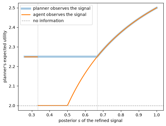
Fig. 31.2 Planner’s value as information improves#
The first-best value \(v\) never falls as \(s\) rises, as Blackwell’s theorem requires, but the planner’s value \(\hat v\) does.
For \(s < 1/3\), both players want \(a_2\) after either refined signal, so the refinement is harmless and useless.
For \(1/3 < s < 2/3\), the players disagree after the signal with posterior \(s\).
The planner then either ignores the agent, which is worth \(2\), or lets him have his way, which is worth \(3 - 1/(2s)\).
So \(\hat v\) jumps down from \(9/4\) to \(2\) at \(s = 1/3\), stays at \(2\) until \(s = 1/2\), and climbs back toward \(9/4\) as \(s\) approaches \(2/3\).
Only for \(s > 2/3\), where the planner and the agent agree again, does the refinement improve the planner’s decisions.
31.8.3. Experiments with two signals#
In Green’s example the harm comes from a refinement that splits one signal into two.
His last result says that this cannot happen when both experiments are binomial channels, Green’s term for experiments with two signals.
Theorem 31.3 (Binomial channels (Green’s Theorem 4))
If \(\Lambda\) is more informative than \(\Lambda'\) and both have two signals, then \(\hat v(\Lambda) \geq \hat v(\Lambda')\), for any number of states and actions.
Here is a proof.
Let \(p_1\) and \(p_2\) be the posteriors of \(\Lambda\), and \(p'_1\) and \(p'_2\) those of \(\Lambda'\).
By (31.3), each \(p'_{n'}\) is an average of \(p_1\) and \(p_2\), so both lie on the segment joining \(p_1\) and \(p_2\).
If \(p'_1 = p'_2\), then \(\Lambda'\) is uninformative, \(\hat v(\Lambda') = v_0\), and there is nothing to prove.
Otherwise, label the signals of \(\Lambda'\) so that \(p'_1\) is closer to \(p_1\) than \(p'_2\) is.
Let \(Z\) be an optimal plan under \(\Lambda'\), and let \(\ell_1\) and \(\ell_2\) be its rows, the lotteries after reports \(y'_1\) and \(y'_2\).
Use the same plan under \(\Lambda\), taking lottery \(\ell_n\) after report \(y_n\).
At a posterior \(p\), the agent’s gain from the lottery \(\ell_1\) over the lottery \(\ell_2\) is \(\phi(p) = (\ell_1 - \ell_2) W p\), and the planner’s is \(\psi(p) = (\ell_1 - \ell_2) U p\).
Both are linear in \(p\).
Truth-telling under \(\Lambda'\) means \(\phi(p'_1) \geq 0 \geq \phi(p'_2)\). The four posteriors lie on the segment in the order \(p_1, p'_1, p'_2, p_2\), so a linear function with these signs at \(p'_1\) and \(p'_2\) keeps them at \(p_1\) and \(p_2\). Hence \(\phi(p_1) \geq 0 \geq \phi(p_2)\), and the plan makes truthful reports optimal under \(\Lambda\).
Optimality of \(Z\) under \(\Lambda'\) implies \(\psi(p'_1) \geq 0 \geq \psi(p'_2)\). For if \(\psi(p'_1) < 0\), the planner would do better by using the lottery \(\ell_2\) after both reports, a plan that ignores the agent and so satisfies the truth-telling constraints; similarly if \(\psi(p'_2) > 0\). By the argument of step 1, \(\psi(p_1) \geq 0 \geq \psi(p_2)\).
Let \(J\) be the joint distribution of the two signals in (31.3). Since \(q'_{n'} p'_{n'} = \sum_n J_{nn'} \, p_n\) and \(q_n = \sum_{n'} J_{nn'}\), the planner’s expected utility from the plan under \(\Lambda\) minus that under \(\Lambda'\) is
\[ \sum_n q_n \ell_n U p_n - \sum_{n'} q'_{n'} \ell_{n'} U p'_{n'} = \sum_{n, n'} J_{nn'} (\ell_n - \ell_{n'}) U p_n = J_{12} \, \psi(p_1) - J_{21} \, \psi(p_2) \;\geq\; 0 . \]
The planner can do at least as well as this plan under \(\Lambda\), so \(\hat v(\Lambda) \geq \hat v(\Lambda')\).
Note
Green’s proof follows the same route, but it has two gaps.
First, it labels the signals so that each row of the garbling \(B\) has its largest entry on the diagonal.
That is not always possible: for \(B = \begin{bmatrix} 0.9 & 0.1 \\ 0.6 & 0.4 \end{bmatrix}\), both rows have their largest entry in the same column, whatever the labels.
The labeling that the argument needs is the one used above, which is equivalent to \(b_{11} \geq b_{21}\), that is, \(\det B \geq 0\).
Second, Green’s last step applies to the planner’s payoffs a sign property that his preceding lemma proves only for the agent’s; step 2 above supplies it from the optimality of \(Z\).
To check the theorem numerically, we draw random binomial channels with up to four states and three or four actions.
We keep only draws in which the theorem does some work.
If \(\hat v(\Lambda') = v_0\) or \(\hat v(\Lambda) = v(\Lambda)\), the conclusion follows from \(v_0 \leq \hat v \leq v\) and Blackwell’s theorem alone, so we skip those draws.
With two actions, Corollary 31.1 says that \(\hat v\) is either \(v_0\) or \(v\), so, if the theorem holds, every draw would be skipped; that is why we use three or four actions.
rng = np.random.default_rng(4321)

gains, tries = [], 0
while len(gains) < 100:
    tries += 1
    M, K = rng.integers(2, 5), rng.integers(3, 5)
    U, W, Λ, π = random_economy(M, K, 2, rng)
    if not plans_differ(U, W, Λ, π):         # then v_hat(Λ) = v(Λ)
        continue
    Λ_prime = Λ @ rng.dirichlet(np.ones(2), size=2)
    v_hat_prime = solve_planner(U, W, Λ_prime, π)[1]
    if v_hat_prime < no_info_value(U, π) + 1e-8:
        continue
    v_hat = solve_planner(U, W, Λ, π)[1]
    if v_hat > bayes_value(U, Λ, π) - 1e-8:
        continue
    gains.append(v_hat - v_hat_prime)
print(f"{len(gains)} informative draws out of {tries}")
print(f"smallest gain from better information: {min(gains):.4f}")
100 informative draws out of 10076
smallest gain from better information: 0.0080
The planner gains from better information in every one of these draws.
When the finer experiment has three or more signals the theorem does not apply, but a loss still requires the players to disagree at some posterior of the finer experiment, as they do at \(s\) when \(1/3 < s < 2/3\); otherwise the planner attains \(\hat v(\Lambda) = v(\Lambda) \geq v(\Lambda') \geq \hat v(\Lambda')\).
31.9. What the discussants added#
Postlewaite [1982] builds four-state examples, his Cases I to IV, in which a more informative experiment helps both players, hurts both, helps the agent and hurts the planner, or helps the planner and hurts the agent.
Exercise 31.2 checks them with the linear program.
In our random draws, Cases I and IV always come out as he says.
In Case II, with \(h\) close to \(j\) as Postlewaite assumes, the agent loses in every draw, but the planner loses in only about half of them.
In Case III the agent loses rather than gains in every draw, while the planner gains in some draws and loses in others.
Postlewaite asks why the agent cannot simply ignore better information, and answers that the planner, knowing that the agent is informed, can design her plan so that an agent who ignored the information would be even worse off.
As we saw after Green’s third example, under a fixed plan better information cannot hurt the agent, so “even worse off” always holds weakly.
In his examples it holds only weakly: Exercise 31.2 studies a family of plans that contains the planner’s optimal plan in both the Case II and the Case III example, and shows that, under her preferred plan in that family, an agent who ignored the finer information would get exactly what he gets by using it.
The agent loses only because the planner, knowing that he is better informed, chooses a different plan; that is why Postlewaite adds that the agent would like to commit to the less informative experiment, if he could convince the planner that he had done so.
Postlewaite also asks who chooses the experiment, and what happens if the agent rather than the planner commits first.
He asserts that it is easy to construct examples in which both players are better off with the roles reversed; Exercise 31.3 confirms this when the agent commits to a deterministic response rule, as Green defines it.
Riley [1982] explains Green’s examples with diagrams of expected utility against the posterior, like Fig. 31.1, and gives a two-state example in which unscrambling a garbled message makes both players worse off.
He concludes that “we cannot expect to obtain more than a multitude of special cases unless the model is refined in some way,” and suggests two refinements.
One is to pay the agent “a fee contingent upon the eventual state of nature.”
The other is to account for “the repetitive nature of informational exchanges,” because long-term relationships, such as those between brokers and clients or physicians and patients, let each party learn the other’s interests.
Repetition can also let reputation stand in for commitment, though Credible Government Policies shows that reputation can support many outcomes, not only the one that commitment would deliver.
Exercise 31.1 shows that, when utilities are linear in money, a fee contingent on the state alone cannot change the agent’s reports, while pay contingent on both the report and the state reduces, but in Riley’s example does not remove, the harm from better information.
31.10. Relation to other lectures#
The Design and Price of Information studies a seller who designs and prices Blackwell experiments and screens buyers, whose prior beliefs are private, with a menu of experiments.
Green’s planner also screens with a menu, but the menu offers lotteries over the planner’s own actions and the private information is the agent’s signal.
In Information and Market Equilibrium, an outside observer can infer an insider’s private information from the equilibrium price, so information travels through a market rather than through a report.
In Expected Utilities of Random Responses, the designer of a randomized response survey deliberately makes each answer less informative, so that respondents are willing to answer truthfully.
The designer accepts a garbled but truthful answer over a sharper but untruthful one, much as the planner in Green’s third example prefers an agent with the coarser experiment.
Green’s planner cannot pay the agent, so she buys truthful reports with distortions in her own actions.
When transfers are available, as in the Groves–Clarke mechanism of Multiple Good Allocation Mechanisms and Groves [1973], payments can do that job instead; Exercise 31.1 adds them to Green’s model.
31.10.1. Later work on communication and delegation#
Green’s model belongs to a family of models of strategic communication that differ in who commits to what.
In the language of this literature, the agent is the sender and the planner the receiver.
In Green’s model the receiver commits to a plan for acting on reports.
In the cheap-talk model of Crawford and Sobel [1982], no one commits, and the receiver acts optimally on whatever she hears.
In the persuasion model of Kamenica and Gentzkow [2011], the sender commits to the experiment that generates the signal.
In Postlewaite’s reversal, studied in Exercise 31.3, the sender commits to a deterministic rule for reporting what he has observed, which is persuasion restricted to partitions of the signals of \(\Lambda\); if the rule may randomize, it is persuasion restricted to garblings of \(\Lambda\).
Riley’s reading of Green’s plan as a menu connects it to the delegation problem of Holmström [1984], in which a principal chooses a set of actions and lets the agent pick one; Green’s menu contains lotteries over actions instead.
Melumad and Shibano [1991] study communication with and without commitment when transfers are ruled out, and Alonso and Matouschek [2008] characterize the optimal set of actions to delegate.
Kováč and Mylovanov [2009] allow randomized plans like Green’s and show that, with quadratic payoffs and a regularity condition, the optimal plan does not randomize.
Green’s finding that the planner can prefer a less informed agent also has descendants.
Fischer and Stocken [2001] show that in cheap talk a less precisely informed sender can leave the receiver better informed, and Ivanov [2010] studies a principal who limits the precision of her agent’s information before he communicates.
31.11. Concluding remarks#
Green’s model separates the person who sees a signal from the person who acts on it.
Commitment lets the planner turn the agent’s incentive problem into a linear program, whose solutions can randomize, use dominated actions as threats, and pool signals.
Because incentive constraints depend on posteriors, the comparison of experiments runs through posteriors as well, and the Marschak–Miyasawa characterization turns Blackwell’s order into a transport problem.
The central lesson concerns the value of information.
Blackwell’s theorem ranks experiments for a decision maker who sees the signal herself, but once the signal must be elicited, a better-informed agent can be worth less to the planner, except when both experiments have only two signals.
31.12. Exercises#
Exercise 31.1
Riley [1982] illustrates how better information can hurt both players with a diagram of a two-state, two-action example, in which he calls signals “messages.”
Here are numbers that reproduce the pattern in his figure C3.4.
Riley’s text names the two actions the other way around from his figure; our labels follow the figure.
The prior is uniform, and with \(p\) the posterior probability of \(\theta_1\), the planner’s expected utilities are \(p\) from \(a_1\) and \(0.7\) from \(a_2\), while the agent’s are \(p\) from \(a_1\) and \((1 - p)/2\) from \(a_2\).
In the coarse experiment the agent’s posterior is \(0.8\) or \(0.2\), each with probability \(1/2\).
In the fine experiment the signal with posterior \(0.2\) is unscrambled into signals with posteriors \(0.4\) and \(0\), each with probability \(1/4\).
Use
garblingto confirm that the fine experiment is more informative than the coarse one. Then solve the planner’s linear program under both experiments, compare both players’ expected utilities, and use Theorem 31.2 to explain the result.Riley suggests paying the agent “a fee contingent upon the eventual state of nature.” Assume that both players’ utilities are linear in money, so that a payment adds to the agent’s utility and subtracts from the planner’s. Show that payments that depend only on the state cannot change the agent’s reports.
Now let the planner pay the agent \(t(r, \theta) \geq 0\) when he reports \(y_r\) and the state turns out to be \(\theta\). Extend the linear program to choose the plan and the payments together, and solve it for the fine experiment. Do the same when payments can depend only on the report. Does pay remove the harm from better information?
Solution
Here is one solution.
For part 1, we build the two experiments, check the garbling, and solve the linear program under each.
π_ri = np.array([1/2, 1/2])
U_ri = np.array([[1.0, 0.0],
                 [0.7, 0.7]])
W_ri = np.array([[1.0, 0.0],
                 [0.0, 0.5]])
Λ_ri_coarse = experiment([0.8, 0.2], [1/2, 1/2], π_ri)
Λ_ri_fine = experiment([0.8, 0.4, 0.0], [1/2, 1/4, 1/4], π_ri)

print("B =\n", garbling(Λ_ri_fine, Λ_ri_coarse, π_ri))
print("reverse garbling:", garbling(Λ_ri_coarse, Λ_ri_fine, π_ri))

for name, Λ in (("coarse", Λ_ri_coarse), ("fine", Λ_ri_fine)):
    Z, v_hat, agent = solve_planner(U_ri, W_ri, Λ, π_ri)
    print(f"{name}: planner {v_hat:.4f}, agent {agent:.4f}, plan\n{Z}")

print(f"fine, agent's first-best plan: "
      f"planner {agent_plan_value(U_ri, W_ri, Λ_ri_fine, π_ri):.4f}, "
      f"agent {bayes_value(W_ri, Λ_ri_fine, π_ri):.4f}")
B =
 [[1. 0.]
 [0. 1.]
 [0. 1.]]
reverse garbling: None
coarse: planner 0.7500, agent 0.6000, plan
[[1. 0.]
 [0. 1.]]
fine: planner 0.7000, agent 0.2500, plan
[[0. 1.]
 [0. 1.]
 [0. 1.]]
fine, agent's first-best plan: planner 0.6750, agent 0.6250
Under the coarse experiment the players agree after both signals: both want \(a_1\) at \(0.8\) and \(a_2\) at \(0.2\).
So the planner gets \(0.75\) and the agent \(0.6\).
Under the fine experiment they disagree at the posterior \(0.4\), where the planner wants \(a_2\) and the agent wants \(a_1\).
By Theorem 31.2, the planner either lets the agent have his way, which is worth \(0.675\) to her and \(0.625\) to him, or ignores him, which is worth \(0.7\) to her.
She ignores him and always takes \(a_2\), which leaves the agent only \(0.25\).
Unscrambling the signal makes both players worse off, as in Riley’s figure.
The figure below has the same structure as Riley’s.
In each panel the solid lines are a player’s expected utilities from the two actions, and the dotted vertical line marks the prior \(1/2\).
Under the coarse experiment the planner takes \(a_2\) at \(0.2\) and \(a_1\) at \(0.8\), so each player’s expected utility is the height at the prior of the dashed chord joining that player’s utilities at those two posteriors (filled dot).
Under the fine experiment the planner always takes \(a_2\), so each player’s expected utility is the height of that player’s line for \(a_2\) at the prior (open dot).
fig, axes = plt.subplots(1, 2, figsize=(10, 4))
for ax, mat, who in zip(axes, (U_ri, W_ri), ("planner", "agent")):
    for k in range(2):
        ax.plot(p_grid, mat[k, 0] * p_grid + mat[k, 1] * (1 - p_grid),
                lw=2, label=f"$a_{k+1}$")
    # coarse experiment: a_2 at the posterior 0.2 and a_1 at the posterior 0.8
    ends = [mat[1] @ [0.2, 0.8], mat[0] @ [0.8, 0.2]]
    ax.plot([0.2, 0.8], ends, "k--", lw=1)
    ax.plot(0.5, np.mean(ends), "ko", label="coarse experiment")
    # fine experiment: a_2 after every signal
    ax.plot(0.5, mat[1] @ [0.5, 0.5], "o", mfc="white", mec="k",
            label="fine experiment")
    ax.axvline(0.5, color="0.6", lw=1, ls=":")
    ax.set_xlabel(r"posterior probability of $\theta_1$")
    ax.set_ylabel(f"expected utility of the {who}")
    ax.legend()
plt.tight_layout()
plt.show()
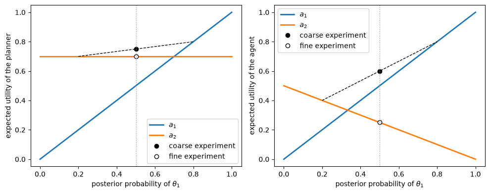
In both panels the open dot lies below the filled dot: \(0.70\) against \(0.75\) for the planner and \(0.25\) against \(0.6\) for the agent.
For part 2, a payment \(t(\theta_m)\) in state \(\theta_m\) adds \(t(\theta_m)\) to every entry in column \(m\) of \(W\).
After observing \(y_n\), the agent then gets an extra \(\sum_m p_{mn} t(\theta_m)\) from every report, so the payment does not change which report is best.
More fundamentally, it does not change the agent’s ranking of actions in any state, so it cannot reduce the conflict between him and the planner.
To change the agent’s incentives, pay has to depend on something that he controls, such as his report.
For part 3, we add the payments to the decision vector.
Pay that depends on the report \(r\) and the state adds \(\sum_m p_{mn} t(r, \theta_m)\) to the agent’s expected utility from report \(y_r\) after signal \(y_n\); pay that depends only on the report adds \(t(r)\).
So the truth-telling constraints and the planner’s expected payment are still linear.
Some payments, such as one after the report with posterior \(0\) in state \(\theta_1\), are never made when the agent tells the truth, so they cost the planner nothing and are not pinned down; a tiny cost on every payment breaks the tie in favor of zero.
def solve_with_pay(U, W, Λ, π, on_state):
    """
    Green's linear program when the planner can also pay the agent.

    If on_state is True the planner pays t[r, m] >= 0 when the agent
    reports y_r and the state is θ_m; otherwise she pays t[r] >= 0 after
    report y_r. Returns the plan, the payments, and the planner's
    expected utility net of expected payments.
    """
    q, P = posteriors(Λ, π)
    K, N = U.shape[0], Λ.shape[1]
    UP, WP = U @ P, W @ P
    # S[l, n] is the probability of payment contingency l after signal n
    S = P if on_state else np.ones((1, N))
    L = S.shape[0]

    # z_{nk} sits at n * K + k, then t[r, l] at N * K + r * L + l
    expected_pay = (S * q).T.ravel()
    c = np.concatenate([-(UP * q).T.ravel(), expected_pay + 1e-9])
    rows = []
    for n in range(N):
        for r in range(N):
            if r != n:
                row_z, row_t = np.zeros((N, K)), np.zeros((N, L))
                row_z[r] += WP[:, n]
                row_z[n] -= WP[:, n]
                row_t[r] += S[:, n]
                row_t[n] -= S[:, n]
                rows.append(np.concatenate([row_z.ravel(), row_t.ravel()]))
    A_ub = np.array(rows).reshape(-1, N * (K + L))
    A_eq = np.hstack([np.kron(np.eye(N), np.ones(K)), np.zeros((N, N * L))])
    res = linprog(c, A_ub=A_ub, b_ub=np.zeros(len(A_ub)),
                  A_eq=A_eq, b_eq=np.ones(N), bounds=(0, None),
                  method="highs", options={"presolve": False})
    if res.status != 0:
        raise RuntimeError(res.message)
    x = np.maximum(res.x, 0.0) + 0.0
    Z = x[:N * K].reshape(N, K)
    t = x[N * K:].reshape(N, L)
    planner = (UP * q).T.ravel() @ x[:N * K] - expected_pay @ x[N * K:]
    return Z, t, planner


for on_state, name in ((True, "report and state"), (False, "report only")):
    Z, t, v_net = solve_with_pay(U_ri, W_ri, Λ_ri_fine, π_ri, on_state)
    print(f"pay on the {name}: planner {v_net:.4f}\nplan\n{Z}\npayments\n{t}")
pay on the report and state: planner 0.7250
plan
[[1. 0.]
 [0. 1.]
 [0. 1.]]
payments
[[0.   0.  ]
 [0.25 0.  ]
 [0.   0.  ]]
pay on the report only: planner 0.7167
plan
[[1.     0.    ]
 [0.1667 0.8333]
 [0.     1.    ]]
payments
[[0.    ]
 [0.0833]
 [0.    ]]
With pay on the report and the state, the planner announces her first-best plan and pays \(0.25\) when the agent reports the posterior \(0.4\) and the state turns out to be \(\theta_1\).
An agent who has seen \(0.4\) expects \(0.4 \times 0.25 = 0.1\) from that payment, exactly his gain \(0.4 - 0.3\) from claiming to have seen \(0.8\).
The payment is cheap because it is aimed at him: an agent who has seen \(0\) expects nothing from it, and one who has seen \(0.8\) is not tempted.
The expected payment is \((1/4)(0.4)(0.25) = 0.025\), so the planner gets \(0.725\).
With pay on the report alone, the planner pays \(1/12\) after report \(0.4\) and also takes \(a_1\) there with probability \(1/6\), for a net value of \(43/60 \approx 0.717\).
Either way, pay shrinks the harm from better information but does not remove it: both values lie between the \(0.70\) the planner gets without pay and the \(0.75\) she gets under the coarse experiment, where no pay is needed.
Two features of these payments matter.
Pay that depends on the state requires that the state be observed afterward, as a stock’s return is.
And the payments must be nonnegative: Green’s model has no participation constraint, so without that restriction the planner could charge the agent an arbitrarily large fee, and the linear program would be unbounded.
Exercise 31.2
Postlewaite [1982] studies four equally likely states \(\theta_1, \ldots, \theta_4\) and four actions.
With positive parameters \(b, c, d, e\) for the planner and \(f, g, h, j\) for the agent, the payoff matrices (rows are actions, columns are states) are
In the fine experiment the agent observes the state.
In the coarse experiment he learns only whether the state is in \(\{\theta_1, \theta_2\}\) or in \(\{\theta_3, \theta_4\}\).
Postlewaite’s Case II assumes \(b > d + e > (b + c)/2 > c\) and \(f > h + j > (f + g)/2 > g\), and he concludes that “if the assumed inequalities hold and also if \(h\) is sufficiently close to \(j\),” the fine experiment leaves both players worse off. Take \((b, c, d, e) = (10, 4, 5, 3)\) and \((f, g, h, j) = (10, 4.5, 3.9, 4)\). Use
garblingto confirm that the fine experiment is more informative than the coarse one. Solve the planner’s linear program under both experiments, and compare both players’ expected utilities. How much probability does the optimal plan under the fine experiment put on actions \(a_3\) and \(a_4\), which are dominated for the planner when \(b > d\) and \(c > e\)?Consider plans under the fine experiment that take \(a_1\) with probability \(x\) and \(a_3\) otherwise after reports \(\theta_1\) and \(\theta_3\), and \(a_2\) with probability \(x\) and \(a_4\) otherwise after reports \(\theta_2\) and \(\theta_4\). Show that truthful reporting is optimal if and only if \(x \leq x^* = \min\{h/(h + g), \, j/(j + f)\}\), and find both players’ expected utilities as functions of \(x\). Postlewaite writes that the probability that can be placed on \(a_1\) and \(a_2\) “becomes arbitrarily small as \(h\) gets arbitrarily close to \(j\).” Is that right?
Postlewaite’s Case III assumes \(b > c > d > e\), \(b > d + e\), \(f > g > j > h\), and \(f < j + h\), and he concludes that, when \(h\) is very close to \(j\), under the fine experiment “the agent is better off and the principal worse off.” Solve the linear program for \((b, c, d, e) = (10, 6, 4, 3)\) and \((f, g, h, j) = (10, 8, 5.9, 6)\). Then show that, under the Case III inequalities, the plan in the family of part 2 that the planner prefers gives the agent less than he gets under the coarse experiment.
Postlewaite’s Case I assumes \(e > d > b > c\) and \(j > h > f > g\), and he concludes that better information helps both players. His Case IV assumes \(b > c > d > e\), \(b < d + e\), \(f > g > j > h\), and \(f > j + h\), and he concludes that, when \(h\) is close to \(j\), it helps the planner and hurts the agent. For each of the four cases, draw many parameter vectors uniformly from \([0, 10]^8\) subject to the case’s inequalities, with \(h\) within \(0.1\) of \(j\) in Cases II to IV, and record how often each player gains or loses. Since the planner may have several optimal plans, compare the agent’s payoffs across all of them. Which of Postlewaite’s four conclusions hold in every draw?
Solution
Here is one solution.
We build the payoff matrices and the two experiments.
Under the coarse experiment the likelihood matrix sends states \(\theta_1\) and \(\theta_2\) to the first signal and states \(\theta_3\) and \(\theta_4\) to the second, so it is also the garbling.
def postlewaite(b, c, d, e, f, g, h, j):
    """Payoffs in Postlewaite's example (rows: actions, columns: states)."""
    U = 2 * np.array([[b, 0, c, 0],
                      [0, c, 0, b],
                      [d, 0, e, 0],
                      [0, e, 0, d]], dtype=float)
    W = 2 * np.array([[0, f, 0, g],
                      [g, 0, f, 0],
                      [h, 0, j, 0],
                      [0, j, 0, h]], dtype=float)
    return U, W


π_pw = np.full(4, 1/4)
Λ_pw_fine = np.eye(4)
Λ_pw_coarse = np.array([[1.0, 0.0],
                        [1.0, 0.0],
                        [0.0, 1.0],
                        [0.0, 1.0]])

print("B =\n", garbling(Λ_pw_fine, Λ_pw_coarse, π_pw))
B =
 [[1. 0.]
 [1. 0.]
 [0. 1.]
 [0. 1.]]
The next function reports the planner’s value and the range of the agent’s expected utility across the planner’s optimal plans, and compare prints them for both experiments.
def payoffs(U, W, Λ, π):
    """
    Planner's value, the agent's lowest and highest payoffs across the
    planner's optimal plans (up to the tolerance in solve_planner), and a
    plan that gives the highest.
    """
    _, v_hat, agent_lo = solve_planner(U, W, Λ, π, ties="agent_worst")
    Z, _, agent_hi = solve_planner(U, W, Λ, π, ties="agent_best")
    return v_hat, agent_lo, agent_hi, Z


def compare(params):
    """Print both players' payoffs; return the plan for the fine experiment."""
    U, W = postlewaite(**params)
    for name, Λ in (("coarse", Λ_pw_coarse), ("fine", Λ_pw_fine)):
        v_hat, lo, hi, Z = payoffs(U, W, Λ, π_pw)
        agent = f"{lo:.4f}" if np.isclose(lo, hi) else f"{lo:.4f} to {hi:.4f}"
        print(f"{name}: planner {v_hat:.4f}, agent {agent}")
    return Z


case_2 = dict(b=10, c=4, d=5, e=3, f=10, g=4.5, h=3.9, j=4)
Z_fine = compare(case_2)
print("optimal plan under the fine experiment:\n", Z_fine)
coarse: planner 10.0000, agent 10.0000
fine: planner 9.7143, agent 5.6429
optimal plan under the fine experiment:
 [[0.2857 0.     0.7143 0.    ]
 [0.     0.2857 0.     0.7143]
 [0.2857 0.     0.7143 0.    ]
 [0.     0.2857 0.     0.7143]]
Under the coarse experiment the plan “\(a_1\) after the first signal, \(a_2\) after the second” gives the planner \(b = 10\) and the agent \(f = 10\), the largest expected payoffs available to either of them under that experiment.
Under the fine experiment the planner gets about \(9.71\) and the agent about \(5.64\), so both lose.
The optimal plan under the fine experiment puts probability \(5/7 \approx 0.71\) on the dominated actions \(a_3\) and \(a_4\), which Postlewaite describes as “placing most of the probability on \(a_3\) and \(a_4\).”
For part 2, an agent who sees \(\theta_1\) gets \(2h(1 - x)\) from the truth and \(2gx\) from reporting \(\theta_2\) or \(\theta_4\).
Reporting \(\theta_3\) gives the same lottery as the truth.
So he reports truthfully if and only if \(h(1 - x) \geq g x\), that is, \(x \leq h/(h + g)\).
Similarly, in state \(\theta_4\) truth requires \(x \leq h/(h + g)\), and in states \(\theta_2\) and \(\theta_3\) it requires \(j(1 - x) \geq f x\), that is, \(x \leq j/(j + f)\).
The planner’s expected utility is \((b + c) x + (d + e)(1 - x)\), which rises with \(x\) when \(b + c > d + e\), so she sets \(x = x^*\).
The agent’s expected utility is \((h + j)(1 - x)\).
def family_values(b, c, d, e, f, g, h, j):
    """x*, and both players' payoffs at x*, in the family of part 2."""
    x_star = min(h / (h + g), j / (j + f))
    planner = (b + c) * x_star + (d + e) * (1 - x_star)
    return x_star, planner, (h + j) * (1 - x_star)


x_star, v_family, a_family = family_values(**case_2)
print(f"x* = {x_star:.4f}, planner {v_family:.4f}, agent {a_family:.4f}")
x* = 0.2857, planner 9.7143, agent 5.6429
These match the linear program.
When an agent who sees \(\theta_1\) lies, he gets a lottery over \(a_2\) and \(a_4\), which pay him \(2g\) and \(0\) in that state, so his truth-telling constraint compares \(h\) with \(g\), and \(j\) does not enter it.
So the bound \(x^*\) depends on how \(h\) compares with \(g\) and how \(j\) compares with \(f\), not on how \(h\) compares with \(j\).
So Postlewaite’s claim is not right: the weight on \(a_1\) and \(a_2\) stays bounded away from zero as \(h\) approaches \(j\), and here it is \(2/7\).
An agent who knows only which pair of states occurred gets \(\max\{xf + (1-x)h, \, xg + (1-x)j\}\) under such a plan.
At \(x = x^*\) this equals \((1 - x^*)(h + j)\), exactly what the informed agent gets.
If \(x^* = j/(j + f)\), as in this example, the first term equals \((1 - x^*)(h + j)\) and the second is no larger, because \(x^* \leq h/(h + g)\); if \(x^* = h/(h + g)\), the roles of the two terms are reversed.
So under the planner’s preferred plan in the family, ignoring the finer information would leave the agent exactly as well off, not worse off.
For part 3, we solve Case III and compare with the family of part 2.
case_3 = dict(b=10, c=6, d=4, e=3, f=10, g=8, h=5.9, j=6)
compare(case_3)
x_star, v_family, a_family = family_values(**case_3)
print(f"family of part 2: x* = {x_star:.4f}, planner {v_family:.4f}, "
      f"agent {a_family:.4f}")
coarse: planner 10.0000, agent 10.0000
fine: planner 10.3750, agent 7.4375
family of part 2: x* = 0.3750, planner 10.3750, agent 7.4375
Under the coarse experiment both players get \(10\), while under the fine experiment the planner gets \(10.375\) and the agent \(7.4375\): the planner gains and the agent loses, the opposite of Postlewaite’s conclusion.
In fact, whenever the Case III inequalities hold, the agent loses under the plan in the family of part 2 that the planner prefers.
Since \(b > d + e\), the planner sets \(x = x^*\).
Under the coarse experiment the agent gets \(f\), and under that plan he gets \((h + j)(1 - x^*)\).
Plans with smaller \(x\) would give him more, up to \(h + j > f\) at \(x = 0\), but the planner does not choose them.
If \(x^* = h/(h + g)\), his payoff is \((h + j) g/(h + g)\), which is less than \(f\) because \(g(j - f) < 0 < h(f - g)\).
If \(x^* = j/(j + f)\), his payoff is \((h + j) f/(j + f)\), which is less than \(f\) because \(h < f\).
Postlewaite’s argument breaks down because he treats the weight on \(a_1\) and \(a_2\) as negligible, which amounts to evaluating the agent’s payoff near \(x = 0\).
For part 4, we draw parameters for each case.
For Cases I, III, and IV, sorting uniform draws gives a uniform draw from the region where they are ordered, which is much faster than rejecting unordered draws.
In Cases II to IV we draw \(h\) within \(0.1\) of \(j\).
def draw_case(case, rng, gap=0.1):
    """
    Uniform draw from [0, 10]^8 subject to the inequalities of a case and,
    in Cases II to IV, to h being within gap of j.
    """
    def decreasing(n):
        return np.sort(rng.uniform(0, 10, n))[::-1]
    while True:
        if case == "I":
            e, d, b, c = decreasing(4)
            j, h, f, g = decreasing(4)
            ok = True
        elif case == "II":
            b, c, d, e, f, g, j = rng.uniform(0, 10, 7)
            h = j + rng.uniform(-gap, gap)
            ok = (0 < h < 10 and b > d + e > (b + c) / 2 > c
                  and f > h + j > (f + g) / 2 > g)
        else:
            b, c, d, e = decreasing(4)
            f, g, j = decreasing(3)
            h = j - rng.uniform(0, gap)
            if case == "III":
                ok = h > 0 and b > d + e and f < j + h
            else:
                ok = h > 0 and b < d + e and f > j + h
        if ok:
            return dict(b=b, c=c, d=d, e=e, f=f, g=g, h=h, j=j)


tol, n_draws = 1e-6, 300
for case in ("I", "II", "III", "IV"):
    rng = np.random.default_rng(0)
    counts = dict(planner_gains=0, planner_loses=0,
                  agent_gains=0, agent_loses=0)
    for _ in range(n_draws):
        U, W = postlewaite(**draw_case(case, rng))
        v_c, lo_c, hi_c, _ = payoffs(U, W, Λ_pw_coarse, π_pw)
        v_f, lo_f, hi_f, _ = payoffs(U, W, Λ_pw_fine, π_pw)
        counts["planner_gains"] += v_f > v_c + tol
        counts["planner_loses"] += v_f < v_c - tol
        # the agent gains or loses whichever optimal plans are used
        counts["agent_gains"] += lo_f > hi_c + tol
        counts["agent_loses"] += hi_f < lo_c - tol
    shares = ", ".join(f"{k} {v / n_draws:.0%}" for k, v in counts.items())
    print(f"Case {case}: {shares}")
Case I: planner_gains 100%, planner_loses 0%, agent_gains 100%, agent_loses 0%
Case II: planner_gains 53%, planner_loses 47%, agent_gains 0%, agent_loses 100%
Case III: planner_gains 60%, planner_loses 40%, agent_gains 0%, agent_loses 100%
Case IV: planner_gains 100%, planner_loses 0%, agent_gains 0%, agent_loses 100%
Cases I and IV come out as Postlewaite says in every draw: in Case I both players gain, and in Case IV the planner gains and the agent loses.
His argument for Case IV repeats the claim that \(h\) close to \(j\) makes the weight on \(a_1\) and \(a_2\) negligible, which part 2 shows is false.
His conclusion about the planner does not need that claim: under the Case IV inequalities, every plan in the family of part 2 is worth \((b + c)x + (d + e)(1 - x) > b\) to her, since both \(b + c\) and \(d + e\) exceed \(b\).
Family plans also give the agent \((h + j)(1 - x) < f\), but the planner’s optimal plan sometimes lies outside the family, so the agent’s loss rests on the draws.
In Case II, the agent loses in every draw, but the planner gains in about half of them, so “both worse off” holds only for some parameters.
Here is an example that satisfies the Case II inequalities, with \(h\) close to \(j\), in which the planner gains.
case_2_gain = dict(b=10, c=9, d=5, e=4.8, f=10, g=4.5, h=3.9, j=4)
_ = compare(case_2_gain)
coarse: planner 10.0000, agent 10.0000
fine: planner 12.4286, agent 5.6429
The planner rises from \(10\) to about \(12.43\) while the agent falls from \(10\) to about \(5.64\).
Postlewaite’s condition that \(h\) be close to \(j\) matters for the agent’s side of Case II: without it, the agent can gain.
case_2_far = dict(b=9, c=3, d=2.5, e=4, f=8, g=7.8, h=1, j=6.95)
_ = compare(case_2_far)
coarse: planner 9.0000, agent 8.0000
fine: planner 8.5000, agent 10.8500
These parameters satisfy the Case II inequalities, with \(h\) far from \(j\), and the agent rises from \(8\) to \(10.85\) while the planner falls from \(9\) to \(8.5\), the pattern that Postlewaite attributes to Case III.
In Case III, the agent loses in every draw, whichever of the planner’s optimal plans is used, and the planner gains in more than half of them.
Part 3 proves the agent’s loss only for the planner’s preferred plan in the family; the draws suggest that it also holds for the linear program’s optimal plans, some of which lie outside the family.
The shares depend on how the parameters are drawn, so they describe the uniform distribution on each region rather than the cases themselves.
Postlewaite’s broader point survives: better information can make both players worse off, or help one and hurt the other.
Exercise 31.3
Postlewaite [1982] asks what happens if the roles are reversed: the agent commits first to a response rule, and the planner then takes the action she likes best given what she hears.
Postlewaite uses Green’s term, and Green’s response rules are deterministic; part 1 also lets the agent randomize.
Argue that the agent loses nothing by recommending actions that the planner is willing to follow. Write the agent’s problem, when he may also randomize, as a linear program in an \(N \times K\) Markov matrix \(\Gamma = [\gamma_{nk}]\), where \(\gamma_{nk}\) is the probability that the agent recommends \(a_k\) after observing \(y_n\), subject to obedience constraints for the planner. Assume that a planner who is indifferent follows the recommendation.
Solve the linear program for the fine experiment of Riley’s example in Exercise 31.1, for Green’s first example, and for the Case II example of Exercise 31.2. Then find the agent’s best deterministic rule, in which every \(\gamma_{nk}\) is \(0\) or \(1\), by checking all of them. Compare both players’ expected utilities with those when the planner leads.
Postlewaite says that “it is straightforward to construct examples where both principal and agent are better off with the roles of leader-follower reversed.” Do these examples support him?
Solution
Here is one solution.
For part 1, any rule for sending messages leads the planner to some action after each message.
Merge all messages after which she takes the same action \(a_k\) into a single message “take \(a_k\).”
Her posterior after the merged message is an average of her posteriors after the original messages, and she preferred \(a_k\) at each of them, so by linearity she still prefers \(a_k\).
The merged rule produces the same joint distribution of signals and actions, so both players’ expected utilities are unchanged, and a deterministic rule stays deterministic.
The planner follows recommendation \(a_k\) if, for every other action \(a_{k'}\),
and the agent maximizes \(\sum_n q_n \sum_k \gamma_{nk} (WP)_{kn}\) subject to these constraints.
This is the persuasion problem of Kamenica and Gentzkow [2011], except that the agent can only garble his own signal rather than design any experiment he likes.
For part 2, solve_agent_leads solves the linear program and best_deterministic_rule checks every deterministic rule; obedience_rows and leader_payoffs are helpers that both use.
def obedience_rows(U, Λ, π):
    """Rows of the obedience constraints, A @ vec(Γ) <= 0."""
    q, P = posteriors(Λ, π)
    UP = U @ P
    K, N = UP.shape
    # Entry n * K + k of vec(Γ) is γ_{nk}; for each recommended action k
    # and alternative j: sum_n q_n γ_{nk} [(UP)_{jn} - (UP)_{kn}] <= 0
    rows = []
    for k in range(K):
        for j in range(K):
            if j != k:
                row = np.zeros((N, K))
                row[:, k] = q * (UP[j] - UP[k])
                rows.append(row.ravel())
    return np.array(rows)


def leader_payoffs(Γ, U, W, Λ, π):
    """Expected utilities of the planner and the agent under Γ."""
    q, P = posteriors(Λ, π)
    return q @ (Γ * (U @ P).T).sum(axis=1), q @ (Γ * (W @ P).T).sum(axis=1)


def solve_agent_leads(U, W, Λ, π):
    """
    The agent's best randomized recommendation rule.

    Returns the N x K rule Γ and the expected utilities of the planner and
    of the agent under it.
    """
    q, P = posteriors(Λ, π)
    K, N = U.shape[0], Λ.shape[1]
    A_ub = obedience_rows(U, Λ, π)
    res = linprog(-((W @ P) * q).T.ravel(), A_ub=A_ub,
                  b_ub=np.zeros(len(A_ub)),
                  A_eq=np.kron(np.eye(N), np.ones(K)), b_eq=np.ones(N),
                  bounds=(0, None), method="highs",
                  options={"presolve": False})
    if res.status != 0:
        raise RuntimeError(res.message)
    Γ = np.maximum(res.x, 0.0).reshape(N, K) + 0.0
    return (Γ, *leader_payoffs(Γ, U, W, Λ, π))


def best_deterministic_rule(U, W, Λ, π):
    """
    The agent's best deterministic recommendation rule, by enumeration;
    among rules that are equally good for him, the planner's favorite.

    Returns the rule Γ and the expected utilities of the planner and of
    the agent under it.
    """
    K, N = U.shape[0], Λ.shape[1]
    A_ub = obedience_rows(U, Λ, π)
    best = None
    for actions in product(range(K), repeat=N):
        Γ = np.eye(K)[list(actions)]
        if np.any(A_ub @ Γ.ravel() > 1e-12):
            continue
        planner, agent = leader_payoffs(Γ, U, W, Λ, π)
        if (best is None or agent > best[2] + 1e-12
                or (agent > best[2] - 1e-12 and planner > best[1])):
            best = (Γ, planner, agent)
    return best


U_c2, W_c2 = postlewaite(**case_2)
examples = (("Riley", U_ri, W_ri, Λ_ri_fine, π_ri),
            ("Green's first", U_ex1, W_ex1, Λ_ex1, π_ex1),
            ("Case II", U_c2, W_c2, Λ_pw_fine, π_pw))
for name, U, W, Λ, π in examples:
    _, v_lead, a_lead = solve_planner(U, W, Λ, π)
    _, v_rand, a_rand = solve_agent_leads(U, W, Λ, π)
    _, v_det, a_det = best_deterministic_rule(U, W, Λ, π)
    print(f"{name}: planner leads ({v_lead:.4f}, {a_lead:.4f}); "
          f"agent leads, deterministic ({v_det:.4f}, {a_det:.4f}), "
          f"randomized ({v_rand:.4f}, {a_rand:.4f})")
Riley: planner leads (0.7000, 0.2500); agent leads, deterministic (0.7500, 0.6000), randomized (0.7000, 0.6167)
Green's first: planner leads (0.6964, -0.0714); agent leads, deterministic (0.8750, 0.3750), randomized (0.5000, 0.6429)
Case II: planner leads (9.7143, 5.6429); agent leads, deterministic (10.0000, 10.0000), randomized (7.0000, 11.3500)
Each pair lists the planner’s expected utility first and the agent’s second.
With a deterministic rule, the agent’s best choice in Riley’s example and in Green’s first example is to tell the truth.
Committing to the truth lets the planner act on everything he knows, which gives the planner her first-best value, and it gives the agent more than he gets when the planner leads.
In Case II, his best deterministic rule reports only which pair of states occurred, which commits him to the coarse experiment, just as Postlewaite says he would like to do; both players then get \(10\).
In these three examples, a randomized rule lets the agent do better still, at the planner’s expense.
In Riley’s example he recommends \(a_1\) after the posterior \(0.4\) with probability \(2/3\), just often enough that a planner told to take \(a_1\), who then puts probability \(0.7\) on \(\theta_1\), is willing to follow.
In Green’s first example the planner falls to \(v_0 = 0.5\), and in Case II to \(7\).
For part 3, Postlewaite is right for the reversal he describes: with a deterministic response rule, reversing the roles makes both players strictly better off in all three examples.
In these examples, an agent who can also randomize takes the planner’s gain for himself, and the planner is no better off, and sometimes much worse off, than when she leads.
That is not a general rule.
Obedience guarantees the planner at least \(v_0\), because she could always take one action regardless of the recommendation, so when her own plan gives her only \(v_0\), she cannot lose by letting the agent lead, even with a randomized rule.
In Riley’s example she merely breaks even, but in the next example both players gain strictly.
Here is an example with two states, a uniform prior, and a perfectly informative experiment.
U_rv = np.array([[0.0, 2.0],
                 [2.0, 1.0],
                 [3.0, 0.0]])
W_rv = np.array([[2.0, 2.0],
                 [0.0, 0.0],
                 [1.0, 2.0]])
Λ_rv, π_rv = np.eye(2), np.array([1/2, 1/2])

v_lead = solve_planner(U_rv, W_rv, Λ_rv, π_rv)[1]
a_best = solve_planner(U_rv, W_rv, Λ_rv, π_rv, ties="agent_best")[2]
_, v_rand, a_rand = solve_agent_leads(U_rv, W_rv, Λ_rv, π_rv)
print(f"planner leads: planner {v_lead:.4f}, agent at most {a_best:.4f}")
print(f"agent leads, randomized: planner {v_rand:.4f}, agent {a_rand:.4f}")
planner leads: planner 1.5000, agent at most 1.5000
agent leads, randomized: planner 1.7500, agent 1.7500
When the planner leads she gets only \(v_0 = 1.5\), and the agent gets at most \(1.5\); when the agent leads with a randomized rule, both get \(1.75\).
Exercise 31.4
Marschak and Miyasawa [1968] compare several conditions on posterior probabilities.
One, which we call the convex-hull condition, requires every posterior of \(\Lambda'\) to lie in the convex hull of the posteriors of \(\Lambda\).
Another is the existence of a joint distribution \(J\) of the two signals, with marginals \(q\) and \(q'\), that satisfies (31.3); it is equivalent to Blackwell’s order.
Take two states with a uniform prior.
Experiment \(\Lambda\) has posteriors \(0.9\), \(0.5\), and \(0.1\) for \(\theta_1\), with probabilities \(0.05\), \(0.9\), and \(0.05\).
Experiment \(\Lambda'\) has posteriors \(0.7\) and \(0.3\), each with probability \(1/2\).
Show that the convex-hull condition holds for \(\Lambda\) against \(\Lambda'\), but that \(\Lambda\) is not more informative than \(\Lambda'\). Explain why, using the variance of the posterior. Is \(\Lambda'\) more informative than \(\Lambda\)?
The equivocation of an experiment is the expected entropy of the posterior, \(-\sum_n q_n \sum_m p_{mn} \log p_{mn}\). Compute it for both experiments. Marschak and Miyasawa’s Theorem 12.3 says that lower equivocation is necessary but not sufficient for being more informative. Illustrate this by finding two decision makers who rank \(\Lambda\) and \(\Lambda'\) in opposite orders. Compare with the treatment of entropy in Blackwell’s Theorem on Comparing Experiments.
Marschak and Miyasawa’s Theorem 10.1 says that the convex-hull condition is sufficient when \(\Lambda\) has only two signals. Explain why, and check it numerically with two states. How does this relate to the proof of Theorem 31.3?
Solution
Here is one solution.
For part 1, the posteriors of \(\Lambda'\), \(0.7\) and \(0.3\), lie in the interval \([0.1, 0.9]\) spanned by those of \(\Lambda\), so the convex-hull condition holds.
π_mm = np.array([1/2, 1/2])
Λ_mm = experiment([0.9, 0.5, 0.1], [0.05, 0.9, 0.05], π_mm)
Λ_mm_prime = experiment([0.7, 0.3], [1/2, 1/2], π_mm)

print("Λ more informative than Λ':",
      garbling(Λ_mm, Λ_mm_prime, π_mm) is not None)
print("Λ' more informative than Λ:",
      garbling(Λ_mm_prime, Λ_mm, π_mm) is not None)

for name, Λ in (("Λ", Λ_mm), ("Λ'", Λ_mm_prime)):
    q, P = posteriors(Λ, π_mm)
    print(f"variance of the posterior under {name}: {q @ (P[0] - 0.5)**2:.4f}")
Λ more informative than Λ': False
Λ' more informative than Λ: False
variance of the posterior under Λ: 0.0160
variance of the posterior under Λ': 0.0400
\(\Lambda\) is not more informative than \(\Lambda'\).
The convex-hull condition compares only the locations of the posteriors and ignores how likely they are.
Under \(\Lambda\) the posterior is usually \(0.5\), so its variance is \(0.016\), while under \(\Lambda'\) the variance is \(0.04\).
A mean-preserving spread raises the variance, so the distribution of posteriors under \(\Lambda\) cannot be a mean-preserving spread of the distribution under \(\Lambda'\).
What rules it out is the requirement that \(J\) have marginal \(q\).
To write the posterior \(0.7\) as an average of \(0.9\), \(0.5\), and \(0.1\), at least half of the weight must go on \(0.9\), so \(J\) would have to put probability at least \(1/4\) on the posterior \(0.9\), which \(\Lambda\) produces only with probability \(0.05\).
Nor is \(\Lambda'\) more informative than \(\Lambda\): the posteriors \(0.9\) and \(0.1\) of \(\Lambda\) lie outside the convex hull \([0.3, 0.7]\) of the posteriors of \(\Lambda'\).
The convex-hull condition is necessary for Blackwell’s order, because each posterior of the less informative experiment is an average of posteriors of the more informative one, so it fails here, and garbling confirms it.
The two experiments are not comparable.
For part 2, we compute the equivocation of each experiment.
def equivocation(Λ, π):
    """Expected entropy of the posterior."""
    q, P = posteriors(Λ, π)
    logs = np.log(P, where=P > 0, out=np.zeros_like(P))
    return -q @ (P * logs).sum(axis=0)


for name, Λ in (("Λ", Λ_mm), ("Λ'", Λ_mm_prime)):
    print(f"equivocation of {name}: {equivocation(Λ, π_mm):.4f}")
equivocation of Λ: 0.6563
equivocation of Λ': 0.6109
\(\Lambda'\) has the lower equivocation, but it is not more informative than \(\Lambda\).
Consider decision makers who choose between a bet that pays \(1\) in state \(\theta_1\) and loses \(x\) in state \(\theta_2\), and no bet.
The bet is worth taking when the posterior exceeds \(x/(1 + x)\).
def bet_utility(x):
    """Bet paying 1 in θ_1 and losing x in θ_2, against no bet."""
    return np.array([[1.0, -x],
                     [0.0, 0.0]])


for x in (4.0, 1.5):
    U_bet = bet_utility(x)
    print(f"x = {x}: threshold {x / (1 + x):.2f}, "
          f"value with Λ {bayes_value(U_bet, Λ_mm, π_mm):.4f}, "
          f"with Λ' {bayes_value(U_bet, Λ_mm_prime, π_mm):.4f}")
x = 4.0: threshold 0.80, value with Λ 0.0250, with Λ' 0.0000
x = 1.5: threshold 0.60, value with Λ 0.0375, with Λ' 0.1250
A cautious bettor who bets only above a posterior of \(0.8\) values \(\Lambda\), which sometimes delivers the posterior \(0.9\), and gets nothing from \(\Lambda'\).
A bolder bettor with threshold \(0.6\) prefers \(\Lambda'\).
This is Marschak and Miyasawa’s point that equivocation, unlike informativeness, orders all experiments, and so cannot capture the dependence of the value of information on the user’s payoffs.
Blackwell’s Theorem on Comparing Experiments makes the same point in DeGroot’s terms: Blackwell’s order requires the uncertainty reduction to be larger for every concave uncertainty function, not only for entropy.
For part 3, suppose that \(\Lambda\) has two signals with distinct posteriors \(p_1\) and \(p_2\), and that every posterior of \(\Lambda'\) lies on the segment joining them.
Write each posterior \(p'_{n'}\) of \(\Lambda'\) as a mixture of \(p_1\) and \(p_2\), and split signal \(y'_{n'}\) according to the mixture weights.
This gives a joint distribution \(J\) whose columns sum to \(q'\) and which satisfies (31.3).
Its row sums put probabilities on \(p_1\) and \(p_2\) whose average is \(\sum_{n'} q'_{n'} p'_{n'} = \pi\).
Only one distribution on two distinct points has mean \(\pi\), so the row sums are \(q\), and \(\Lambda\) is more informative than \(\Lambda'\).
The requirement that the row sums of \(J\) equal \(q\), which failed in part 1, holds automatically, for any number of states.
We check this by drawing random experiments \(\Lambda'\) and a two-signal \(\Lambda\) whose posteriors bracket those of \(\Lambda'\).
rng = np.random.default_rng(2468)

found = []
for _ in range(500):
    N_prime = rng.integers(2, 6)
    post = rng.uniform(0.05, 0.95, N_prime)
    probs = rng.dirichlet(np.ones(N_prime))
    π = np.array([probs @ post, 1 - probs @ post])
    lo = rng.uniform(0, post.min())
    hi = rng.uniform(post.max(), 1)
    w_hi = (π[0] - lo) / (hi - lo)
    Λ_binary = experiment([hi, lo], [w_hi, 1 - w_hi], π)
    Λ_other = experiment(post, probs, π)
    found.append(garbling(Λ_binary, Λ_other, π) is not None)
print("garbling found in every draw:", all(found))
garbling found in every draw: True
The proof of Theorem 31.3 uses the information order through two facts: the posteriors of \(\Lambda'\) lie on the segment joining those of \(\Lambda\), and there is a joint distribution \(J\) satisfying (31.3).
When \(\Lambda\) has two signals, the argument above shows that the first fact delivers the second, so Blackwell’s order is then a condition on where the posteriors lie, not on how likely they are.