112. Linear Regression in Python#
In addition to what’s in Anaconda, this lecture will need the following libraries:
!pip install linearmodels
112.1. Overview#
Linear regression is a standard tool for analyzing the relationship between two or more variables.
In this lecture, we’ll use the Python package statsmodels to estimate, interpret, and visualize linear regression models.
Along the way, we’ll discuss a variety of topics, including
simple and multivariate linear regression
visualization
endogeneity and omitted variable bias
two-stage least squares
As an example, we will replicate results from Acemoglu, Johnson and Robinson’s seminal paper [Acemoglu et al., 2001].
You can download a copy here.
In the paper, the authors emphasize the importance of institutions in economic development.
The main contribution is the use of settler mortality rates as a source of exogenous variation in institutional differences.
Such variation is needed to determine whether it is institutions that give rise to greater economic growth, rather than the other way around.
Let’s start with some imports:
import matplotlib.pyplot as plt
import numpy as np
import pandas as pd
import statsmodels.api as sm
from statsmodels.iolib.summary2 import summary_col
from linearmodels.iv import IV2SLS
import seaborn as sns
sns.set_theme()
112.1.1. Prerequisites#
This lecture assumes you are familiar with basic econometrics.
For an introductory text covering these topics, see, for example, [Wooldridge, 2015].
112.2. Simple Linear Regression#
[Acemoglu et al., 2001] wish to determine whether or not differences in institutions can help to explain observed economic outcomes.
How do we measure institutional differences and economic outcomes?
In this paper,
economic outcomes are proxied by log GDP per capita in 1995, adjusted for exchange rates.
institutional differences are proxied by an index of protection against expropriation on average over 1985-95, constructed by the Political Risk Services Group.
These variables and other data used in the paper are available for download on Daron Acemoglu’s webpage.
We will use pandas’ .read_stata() function to read in data contained in the .dta files to dataframes
df1 = pd.read_stata('https://github.com/QuantEcon/lecture-python.myst/raw/refs/heads/main/lectures/_static/lecture_specific/ols/maketable1.dta')
df1.head()
| shortnam | euro1900 | excolony | avexpr | logpgp95 | cons1 | cons90 | democ00a | cons00a | extmort4 | logem4 | loghjypl | baseco | |
|---|---|---|---|---|---|---|---|---|---|---|---|---|---|
| 0 | AFG | 0.000000 | 1.0 | NaN | NaN | 1.0 | 2.0 | 1.0 | 1.0 | 93.699997 | 4.540098 | NaN | NaN |
| 1 | AGO | 8.000000 | 1.0 | 5.363636 | 7.770645 | 3.0 | 3.0 | 0.0 | 1.0 | 280.000000 | 5.634789 | -3.411248 | 1.0 |
| 2 | ARE | 0.000000 | 1.0 | 7.181818 | 9.804219 | NaN | NaN | NaN | NaN | NaN | NaN | NaN | NaN |
| 3 | ARG | 60.000004 | 1.0 | 6.386364 | 9.133459 | 1.0 | 6.0 | 3.0 | 3.0 | 68.900002 | 4.232656 | -0.872274 | 1.0 |
| 4 | ARM | 0.000000 | 0.0 | NaN | 7.682482 | NaN | NaN | NaN | NaN | NaN | NaN | NaN | NaN |
Let’s use a scatterplot to see whether any obvious relationship exists between GDP per capita and the protection against expropriation index
df1.plot(x='avexpr', y='logpgp95', kind='scatter')
plt.show()
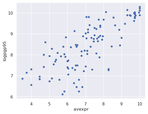
The plot shows a fairly strong positive relationship between protection against expropriation and log GDP per capita.
Specifically, if higher protection against expropriation is a measure of institutional quality, then better institutions appear to be positively correlated with better economic outcomes (higher GDP per capita).
Given the plot, choosing a linear model to describe this relationship seems like a reasonable assumption.
We can write our model as
where:
\(\beta_0\) is the intercept of the linear trend line on the y-axis
\(\beta_1\) is the slope of the linear trend line, representing the marginal effect of protection against risk on log GDP per capita
\(u_i\) is a random error term (deviations of observations from the linear trend due to factors not included in the model)
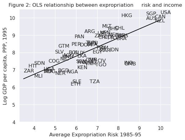
Visually, this linear model involves choosing a straight line that best fits the data, as in the following plot (Figure 2 in [Acemoglu et al., 2001])
# Dropping NA's is required to use numpy's polyfit
df1_subset = df1.dropna(subset=['logpgp95', 'avexpr'])

# Use only 'base sample' for plotting purposes
df1_subset = df1_subset[df1_subset['baseco'] == 1]

X = df1_subset['avexpr']
y = df1_subset['logpgp95']
labels = df1_subset['shortnam']

# Replace markers with country labels
fig, ax = plt.subplots()
ax.scatter(X, y, marker='')

for i, label in enumerate(labels):
    ax.annotate(label, (X.iloc[i], y.iloc[i]))

# Fit a linear trend line
ax.plot(np.unique(X),
         np.poly1d(np.polyfit(X, y, 1))(np.unique(X)),
         color='black')

ax.set_xlim([3.3,10.5])
ax.set_ylim([4,10.5])
ax.set_xlabel('Average Expropriation Risk 1985-95')
ax.set_ylabel('Log GDP per capita, PPP, 1995')
ax.set_title('Figure 2: OLS relationship between expropriation \
    risk and income')
plt.show()
The most common technique to estimate the parameters (\(\beta\)’s) of the linear model is Ordinary Least Squares (OLS).
As the name implies, an OLS model is solved by finding the parameters that minimize the sum of squared residuals, i.e.
where \(\hat{u}_i\) is the difference between the observation and the predicted value of the dependent variable.
To estimate the constant term \(\beta_0\), we need to add a column of 1’s to our dataset (consider the equation if \(\beta_0\) was replaced with \(\beta_0 x_i\) and \(x_i = 1\))
df1['const'] = 1
Now we can construct our model in statsmodels using the OLS function.
We will use pandas dataframes with statsmodels, however standard arrays can also be used as arguments
reg1 = sm.OLS(endog=df1['logpgp95'], exog=df1[['const', 'avexpr']], \
    missing='drop')
type(reg1)
statsmodels.regression.linear_model.OLS
So far we have simply constructed our model.
We need to use .fit() to obtain parameter estimates
\(\hat{\beta}_0\) and \(\hat{\beta}_1\)
results = reg1.fit()
type(results)
statsmodels.regression.linear_model.RegressionResultsWrapper
We now have the fitted regression model stored in results.
To view the OLS regression results, we can call the .summary()
method.
Note that an observation was mistakenly dropped from the results in the
original paper (see the note located in maketable2.do from Acemoglu’s webpage), and thus the
coefficients differ slightly.
print(results.summary())
                            OLS Regression Results
==============================================================================
Dep. Variable:               logpgp95   R-squared:                       0.611
Model:                            OLS   Adj. R-squared:                  0.608
Method:                 Least Squares   F-statistic:                     171.4
Date:                Thu, 16 Jul 2026   Prob (F-statistic):           4.16e-24
Time:                        06:50:10   Log-Likelihood:                -119.71
No. Observations:                 111   AIC:                             243.4
Df Residuals:                     109   BIC:                             248.8
Df Model:                           1
Covariance Type:            nonrobust
==============================================================================
                 coef    std err          t      P>|t|      [0.025      0.975]
------------------------------------------------------------------------------
const          4.6261      0.301     15.391      0.000       4.030       5.222
avexpr         0.5319      0.041     13.093      0.000       0.451       0.612
==============================================================================
Omnibus:                        9.251   Durbin-Watson:                   1.689
Prob(Omnibus):                  0.010   Jarque-Bera (JB):                9.170
Skew:                          -0.680   Prob(JB):                       0.0102
Kurtosis:                       3.362   Cond. No.                         33.2
==============================================================================

Notes:
[1] Standard Errors assume that the covariance matrix of the errors is correctly specified.
From our results, we see that
The intercept \(\hat{\beta}_0 = 4.63\).
The slope \(\hat{\beta}_1 = 0.53\).
The positive \(\hat{\beta}_1\) parameter estimate implies that. institutional quality has a positive effect on economic outcomes, as we saw in the figure.
The p-value of 0.000 for \(\hat{\beta}_1\) implies that the effect of institutions on GDP is statistically significant (using p < 0.05 as a rejection rule).
The R-squared value of 0.611 indicates that around 61% of variation in log GDP per capita is explained by protection against expropriation.
Using our parameter estimates, we can now write our estimated relationship as
This equation describes the line that best fits our data, as shown in Figure 2.
We can use this equation to predict the level of log GDP per capita for a value of the index of expropriation protection.
For example, for a country with an index value of 7.07 (the average for the dataset), we find that their predicted level of log GDP per capita in 1995 is 8.38.
mean_expr = np.mean(df1_subset['avexpr'])
mean_expr
np.float32(6.515625)
predicted_logpdp95 = 4.63 + 0.53 * 7.07
predicted_logpdp95
8.3771
An easier (and more accurate) way to obtain this result is to use
.predict() and set \(constant = 1\) and
\({avexpr}_i = mean\_expr\)
results.predict(exog=[1, mean_expr])
array([8.09156367])
We can obtain an array of predicted \({logpgp95}_i\) for every value
of \({avexpr}_i\) in our dataset by calling .predict() on our
results.
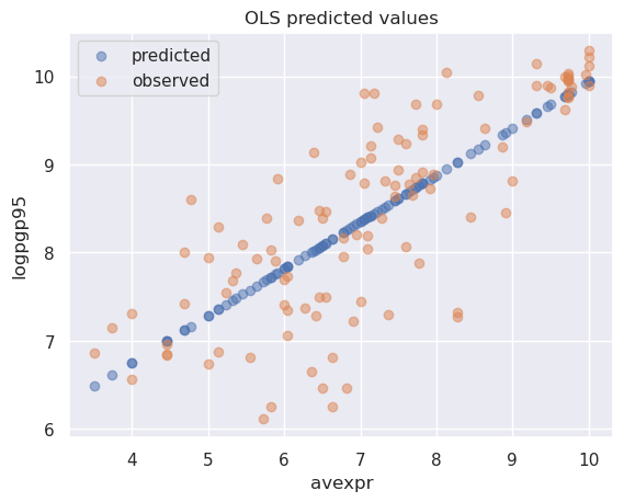
Plotting the predicted values against \({avexpr}_i\) shows that the predicted values lie along the linear line that we fitted above.
The observed values of \({logpgp95}_i\) are also plotted for comparison purposes
# Drop missing observations from whole sample

df1_plot = df1.dropna(subset=['logpgp95', 'avexpr'])

# Plot predicted values

fix, ax = plt.subplots()
ax.scatter(df1_plot['avexpr'], results.predict(), alpha=0.5,
        label='predicted')

# Plot observed values

ax.scatter(df1_plot['avexpr'], df1_plot['logpgp95'], alpha=0.5,
        label='observed')

ax.legend()
ax.set_title('OLS predicted values')
ax.set_xlabel('avexpr')
ax.set_ylabel('logpgp95')
plt.show()
112.3. Extending the Linear Regression Model#
So far we have only accounted for institutions affecting economic performance - almost certainly there are numerous other factors affecting GDP that are not included in our model.
Leaving out variables that affect \(logpgp95_i\) will result in omitted variable bias, yielding biased and inconsistent parameter estimates.
We can extend our bivariate regression model to a multivariate regression model by adding in other factors that may affect \(logpgp95_i\).
[Acemoglu et al., 2001] consider other factors such as:
the effect of climate on economic outcomes; latitude is used to proxy this
differences that affect both economic performance and institutions, eg. cultural, historical, etc.; controlled for with the use of continent dummies
Let’s estimate some of the extended models considered in the paper
(Table 2) using data from maketable2.dta
df2 = pd.read_stata('https://github.com/QuantEcon/lecture-python.myst/raw/refs/heads/main/lectures/_static/lecture_specific/ols/maketable2.dta')

# Add constant term to dataset
df2['const'] = 1

# Create lists of variables to be used in each regression
X1 = ['const', 'avexpr']
X2 = ['const', 'avexpr', 'lat_abst']
X3 = ['const', 'avexpr', 'lat_abst', 'asia', 'africa', 'other']

# Estimate an OLS regression for each set of variables
reg1 = sm.OLS(df2['logpgp95'], df2[X1], missing='drop').fit()
reg2 = sm.OLS(df2['logpgp95'], df2[X2], missing='drop').fit()
reg3 = sm.OLS(df2['logpgp95'], df2[X3], missing='drop').fit()
Now that we have fitted our model, we will use summary_col to
display the results in a single table (model numbers correspond to those
in the paper)
info_dict={'R-squared' : lambda x: f"{x.rsquared:.2f}",
           'No. observations' : lambda x: f"{int(x.nobs):d}"}

results_table = summary_col(results=[reg1,reg2,reg3],
                            float_format='%0.2f',
                            stars = True,
                            model_names=['Model 1',
                                         'Model 3',
                                         'Model 4'],
                            info_dict=info_dict,
                            regressor_order=['const',
                                             'avexpr',
                                             'lat_abst',
                                             'asia',
                                             'africa'])

results_table.add_title('Table 2 - OLS Regressions')

print(results_table)
        Table 2 - OLS Regressions
=========================================
                 Model 1 Model 3 Model 4
-----------------------------------------
const            4.63*** 4.87*** 5.85***
                 (0.30)  (0.33)  (0.34)
avexpr           0.53*** 0.46*** 0.39***
                 (0.04)  (0.06)  (0.05)
lat_abst                 0.87*   0.33
                         (0.49)  (0.45)
asia                             -0.15
                                 (0.15)
africa                           -0.92***
                                 (0.17)
other                            0.30
                                 (0.37)
R-squared        0.61    0.62    0.72
R-squared Adj.   0.61    0.62    0.70
No. observations 111     111     111
R-squared        0.61    0.62    0.72
=========================================
Standard errors in parentheses.
* p<.1, ** p<.05, ***p<.01
112.4. Endogeneity#
As [Acemoglu et al., 2001] discuss, the OLS models likely suffer from endogeneity issues, resulting in biased and inconsistent model estimates.
Namely, there is likely a two-way relationship between institutions and economic outcomes:
richer countries may be able to afford or prefer better institutions
variables that affect income may also be correlated with institutional differences
the construction of the index may be biased; analysts may be biased towards seeing countries with higher income having better institutions
To deal with endogeneity, we can use two-stage least squares (2SLS) regression, which is an extension of OLS regression.
This method requires replacing the endogenous variable \({avexpr}_i\) with a variable that is:
correlated with \({avexpr}_i\)
not correlated with the error term (ie. it should not directly affect the dependent variable, otherwise it would be correlated with \(u_i\) due to omitted variable bias)
The new set of regressors is called an instrument, which aims to remove endogeneity in our proxy of institutional differences.
The main contribution of [Acemoglu et al., 2001] is the use of settler mortality rates to instrument for institutional differences.
They hypothesize that higher mortality rates of colonizers led to the establishment of institutions that were more extractive in nature (less protection against expropriation), and these institutions still persist today.
Using a scatterplot (Figure 3 in [Acemoglu et al., 2001]), we can see protection against expropriation is negatively correlated with settler mortality rates, coinciding with the authors’ hypothesis and satisfying the first condition of a valid instrument.
# Dropping NA's is required to use numpy's polyfit
df1_subset2 = df1.dropna(subset=['logem4', 'avexpr'])

X = df1_subset2['logem4']
y = df1_subset2['avexpr']
labels = df1_subset2['shortnam']

# Replace markers with country labels
fig, ax = plt.subplots()
ax.scatter(X, y, marker='')

for i, label in enumerate(labels):
    ax.annotate(label, (X.iloc[i], y.iloc[i]))

# Fit a linear trend line
ax.plot(np.unique(X),
         np.poly1d(np.polyfit(X, y, 1))(np.unique(X)),
         color='black')

ax.set_xlim([1.8,8.4])
ax.set_ylim([3.3,10.4])
ax.set_xlabel('Log of Settler Mortality')
ax.set_ylabel('Average Expropriation Risk 1985-95')
ax.set_title('Figure 3: First-stage relationship between settler mortality \
    and expropriation risk')
plt.show()
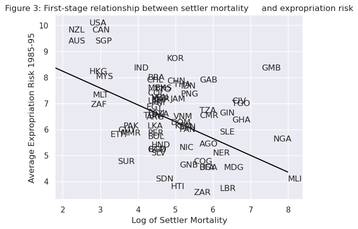
The second condition may not be satisfied if settler mortality rates in the 17th to 19th centuries have a direct effect on current GDP (in addition to their indirect effect through institutions).
For example, settler mortality rates may be related to the current disease environment in a country, which could affect current economic performance.
[Acemoglu et al., 2001] argue this is unlikely because:
The majority of settler deaths were due to malaria and yellow fever and had a limited effect on local people.
The disease burden on local people in Africa or India, for example, did not appear to be higher than average, supported by relatively high population densities in these areas before colonization.
As we appear to have a valid instrument, we can use 2SLS regression to obtain consistent and unbiased parameter estimates.
First stage
The first stage involves regressing the endogenous variable (\({avexpr}_i\)) on the instrument.
The instrument is the set of all exogenous variables in our model (and not just the variable we have replaced).
Using model 1 as an example, our instrument is simply a constant and settler mortality rates \({logem4}_i\).
Therefore, we will estimate the first-stage regression as
The data we need to estimate this equation is located in
maketable4.dta (only complete data, indicated by baseco = 1, is
used for estimation)
# Import and select the data
df4 = pd.read_stata('https://github.com/QuantEcon/lecture-python.myst/raw/refs/heads/main/lectures/_static/lecture_specific/ols/maketable4.dta')
df4 = df4[df4['baseco'] == 1]

# Add a constant variable
df4['const'] = 1

# Fit the first stage regression and print summary
results_fs = sm.OLS(df4['avexpr'],
                    df4[['const', 'logem4']],
                    missing='drop').fit()
print(results_fs.summary())
                            OLS Regression Results
==============================================================================
Dep. Variable:                 avexpr   R-squared:                       0.270
Model:                            OLS   Adj. R-squared:                  0.258
Method:                 Least Squares   F-statistic:                     22.95
Date:                Thu, 16 Jul 2026   Prob (F-statistic):           1.08e-05
Time:                        06:50:11   Log-Likelihood:                -104.83
No. Observations:                  64   AIC:                             213.7
Df Residuals:                      62   BIC:                             218.0
Df Model:                           1
Covariance Type:            nonrobust
==============================================================================
                 coef    std err          t      P>|t|      [0.025      0.975]
------------------------------------------------------------------------------
const          9.3414      0.611     15.296      0.000       8.121      10.562
logem4        -0.6068      0.127     -4.790      0.000      -0.860      -0.354
==============================================================================
Omnibus:                        0.035   Durbin-Watson:                   2.003
Prob(Omnibus):                  0.983   Jarque-Bera (JB):                0.172
Skew:                           0.045   Prob(JB):                        0.918
Kurtosis:                       2.763   Cond. No.                         19.4
==============================================================================

Notes:
[1] Standard Errors assume that the covariance matrix of the errors is correctly specified.
Second stage
We need to retrieve the predicted values of \({avexpr}_i\) using
.predict().
We then replace the endogenous variable \({avexpr}_i\) with the predicted values \(\widehat{avexpr}_i\) in the original linear model.
Our second stage regression is thus
df4['predicted_avexpr'] = results_fs.predict()

results_ss = sm.OLS(df4['logpgp95'],
                    df4[['const', 'predicted_avexpr']]).fit()
print(results_ss.summary())
                            OLS Regression Results
==============================================================================
Dep. Variable:               logpgp95   R-squared:                       0.477
Model:                            OLS   Adj. R-squared:                  0.469
Method:                 Least Squares   F-statistic:                     56.60
Date:                Thu, 16 Jul 2026   Prob (F-statistic):           2.66e-10
Time:                        06:50:11   Log-Likelihood:                -72.268
No. Observations:                  64   AIC:                             148.5
Df Residuals:                      62   BIC:                             152.9
Df Model:                           1
Covariance Type:            nonrobust
====================================================================================
                       coef    std err          t      P>|t|      [0.025      0.975]
------------------------------------------------------------------------------------
const                1.9097      0.823      2.320      0.024       0.264       3.555
predicted_avexpr     0.9443      0.126      7.523      0.000       0.693       1.195
==============================================================================
Omnibus:                       10.547   Durbin-Watson:                   2.137
Prob(Omnibus):                  0.005   Jarque-Bera (JB):               11.010
Skew:                          -0.790   Prob(JB):                      0.00407
Kurtosis:                       4.277   Cond. No.                         58.1
==============================================================================

Notes:
[1] Standard Errors assume that the covariance matrix of the errors is correctly specified.
The second-stage regression results give us an unbiased and consistent estimate of the effect of institutions on economic outcomes.
The result suggests a stronger positive relationship than what the OLS results indicated.
Note that while our parameter estimates are correct, our standard errors are not and for this reason, computing 2SLS ‘manually’ (in stages with OLS) is not recommended.
We can correctly estimate a 2SLS regression in one step using the
linearmodels package, an extension of statsmodels
Note that when using IV2SLS, the exogenous and instrument variables
are split up in the function arguments (whereas before the instrument
included exogenous variables)
iv = IV2SLS(dependent=df4['logpgp95'],
            exog=df4['const'],
            endog=df4['avexpr'],
            instruments=df4['logem4']).fit(cov_type='unadjusted')

print(iv.summary)
                          IV-2SLS Estimation Summary
==============================================================================
Dep. Variable:               logpgp95   R-squared:                      0.1870
Estimator:                    IV-2SLS   Adj. R-squared:                 0.1739
No. Observations:                  64   F-statistic:                    37.568
Date:                Thu, Jul 16 2026   P-value (F-stat)                0.0000
Time:                        06:50:11   Distribution:                  chi2(1)
Cov. Estimator:            unadjusted

                             Parameter Estimates
==============================================================================
            Parameter  Std. Err.     T-stat    P-value    Lower CI    Upper CI
------------------------------------------------------------------------------
const          1.9097     1.0106     1.8897     0.0588     -0.0710      3.8903
avexpr         0.9443     0.1541     6.1293     0.0000      0.6423      1.2462
==============================================================================

Endogenous: avexpr
Instruments: logem4
Unadjusted Covariance (Homoskedastic)
Debiased: False
Given that we now have consistent and unbiased estimates, we can infer from the model we have estimated that institutional differences (stemming from institutions set up during colonization) can help to explain differences in income levels across countries today.
[Acemoglu et al., 2001] use a marginal effect of 0.94 to calculate that the difference in the index between Chile and Nigeria (ie. institutional quality) implies up to a 7-fold difference in income, emphasizing the significance of institutions in economic development.
112.5. Summary#
We have demonstrated basic OLS and 2SLS regression in statsmodels and linearmodels.
If you are familiar with R, you may want to use the formula interface to statsmodels, or consider using r2py to call R from within Python.
112.6. Exercises#
Exercise 112.1
In the lecture, we think the original model suffers from endogeneity bias due to the likely effect income has on institutional development.
Although endogeneity is often best identified by thinking about the data and model, we can formally test for endogeneity using the Hausman test.
We want to test for correlation between the endogenous variable, \(avexpr_i\), and the errors, \(u_i\)
This test is running in two stages.
First, we regress \(avexpr_i\) on the instrument, \(logem4_i\)
Second, we retrieve the residuals \(\hat{\upsilon}_i\) and include them in the original equation
If \(\alpha\) is statistically significant (with a p-value < 0.05), then we reject the null hypothesis and conclude that \(avexpr_i\) is endogenous.
Using the above information, estimate a Hausman test and interpret your results.
Solution
# Load in data
df4 = pd.read_stata('https://github.com/QuantEcon/lecture-python.myst/raw/refs/heads/main/lectures/_static/lecture_specific/ols/maketable4.dta')

# Add a constant term
df4['const'] = 1

# Estimate the first stage regression
reg1 = sm.OLS(endog=df4['avexpr'],
              exog=df4[['const', 'logem4']],
              missing='drop').fit()

# Retrieve the residuals
df4['resid'] = reg1.resid

# Estimate the second stage residuals
reg2 = sm.OLS(endog=df4['logpgp95'],
              exog=df4[['const', 'avexpr', 'resid']],
              missing='drop').fit()

print(reg2.summary())
                            OLS Regression Results
==============================================================================
Dep. Variable:               logpgp95   R-squared:                       0.689
Model:                            OLS   Adj. R-squared:                  0.679
Method:                 Least Squares   F-statistic:                     74.05
Date:                Thu, 16 Jul 2026   Prob (F-statistic):           1.07e-17
Time:                        06:50:11   Log-Likelihood:                -62.031
No. Observations:                  70   AIC:                             130.1
Df Residuals:                      67   BIC:                             136.8
Df Model:                           2
Covariance Type:            nonrobust
==============================================================================
                 coef    std err          t      P>|t|      [0.025      0.975]
------------------------------------------------------------------------------
const          2.4782      0.547      4.530      0.000       1.386       3.570
avexpr         0.8564      0.082     10.406      0.000       0.692       1.021
resid         -0.4951      0.099     -5.017      0.000      -0.692      -0.298
==============================================================================
Omnibus:                       17.597   Durbin-Watson:                   2.086
Prob(Omnibus):                  0.000   Jarque-Bera (JB):               23.194
Skew:                          -1.054   Prob(JB):                     9.19e-06
Kurtosis:                       4.873   Cond. No.                         53.8
==============================================================================

Notes:
[1] Standard Errors assume that the covariance matrix of the errors is correctly specified.
The output shows that the coefficient on the residuals is statistically significant, indicating \(avexpr_i\) is endogenous.
Exercise 112.2
The OLS parameter \(\beta\) can also be estimated using matrix
algebra and numpy (you may need to review the
numpy lecture to
complete this exercise).
The linear equation we want to estimate is (written in matrix form)
To solve for the unknown parameter \(\beta\), we want to minimize the sum of squared residuals
Rearranging the first equation and substituting into the second equation, we can write
Solving this optimization problem gives the solution for the \(\hat{\beta}\) coefficients
Using the above information, compute \(\hat{\beta}\) from model 1
using numpy - your results should be the same as those in the
statsmodels output from earlier in the lecture.
Solution
# Load in data
df1 = pd.read_stata('https://github.com/QuantEcon/lecture-python.myst/raw/refs/heads/main/lectures/_static/lecture_specific/ols/maketable1.dta')
df1 = df1.dropna(subset=['logpgp95', 'avexpr'])

# Add a constant term
df1['const'] = 1

# Define the X and y variables
y = np.asarray(df1['logpgp95'])
X = np.asarray(df1[['const', 'avexpr']])

# Compute β_hat
β_hat = np.linalg.solve(X.T @ X, X.T @ y)

# Print out the results from the 2 x 1 vector β_hat
print(f'β_0 = {β_hat[0]:.2}')
print(f'β_1 = {β_hat[1]:.2}')
β_0 = 4.6
β_1 = 0.53
It is also possible to use np.linalg.inv(X.T @ X) @ X.T @ y to solve
for \(\beta\), however .solve() is preferred as it involves fewer
computations.