20. Forecasting an AR(1) Process#
GPU
This lecture was built using a machine with access to a GPU — although it will also run without one.
Google Colab has a free tier with GPUs that you can access as follows:
Click on the “play” icon top right
Select Colab
Set the runtime environment to include a GPU
!pip install numpyro jax arviz
This lecture describes methods for forecasting statistics that are functions of future values of a univariate autoregressive process.
The methods are designed to take into account two possible sources of uncertainty about these statistics:
random shocks that impinge on the transition law
uncertainty about the parameter values of the AR(1) process
We consider two sorts of statistics:
prospective values \(y_{t+j}\) of a random process \(\{y_t\}\) that is governed by the AR(1) process
sample path properties that are defined as non-linear functions of future values \(\{y_{t+j}\}_{j \geq 1}\) at time \(t\)
Sample path properties are things like “time to next turning point” or “time to next recession”.
To investigate sample path properties we’ll use a simulation procedure recommended by Wecker [Wecker, 1979].
To acknowledge uncertainty about parameters, we’ll deploy numpyro to construct a Bayesian joint posterior distribution for unknown parameters.
This lecture builds on Posterior Distributions for AR(1) Parameters, which studies Bayesian inference for the parameters of exactly this AR(1) model in detail.
We recommend reading that lecture first, since here we treat the construction of the posterior more briefly.
Let’s start with some imports.
import matplotlib.pyplot as plt
import seaborn as sns
from typing import NamedTuple

# numpyro
import numpyro
import numpyro.distributions as dist
from numpyro.infer import MCMC, NUTS

# jax
import jax
import jax.random as random
import jax.numpy as jnp
from jax import lax

# arviz
import arviz as az

sns.set_style('white')
key = random.PRNGKey(0)
Matplotlib is building the font cache; this may take a moment.
20.1. A Univariate First-Order Autoregressive Process#
Consider the univariate AR(1) model, which is the same model studied in Posterior Distributions for AR(1) Parameters:
where
the scalars \(\rho\) and \(\sigma\) satisfy \(|\rho| < 1\) and \(\sigma > 0\)
\(\{\epsilon_{t+1}\}\) is a sequence of IID normal random variables with mean \(0\) and variance \(1\).
The initial condition \(y_{0}\) is a known number.
Equation (20.1) implies that for \(t \geq 0\), the conditional density of \(y_{t+1}\) is
Further, equation (20.1) also implies that for \(t \geq 0\), the conditional density of \(y_{t+j}\) for \(j \geq 1\) is
The predictive distribution (20.3) assumes that the parameters \(\rho, \sigma\) are known, which we express by conditioning on them.
We also want to compute a predictive distribution that does not condition on \(\rho,\sigma\) but instead takes account of our uncertainty about them.
We form this predictive distribution by integrating (20.3) with respect to a joint posterior distribution \(\pi_t(\rho,\sigma | y^t)\) that conditions on an observed history \(y^t = \{y_s\}_{s=0}^t\):
Predictive distribution (20.3) assumes that parameters \((\rho,\sigma)\) are known.
Predictive distribution (20.4) assumes that parameters \((\rho,\sigma)\) are uncertain, but have a known probability distribution \(\pi_t(\rho,\sigma | y^t )\). Notice the second equality follows because \(\{y_t\}\) is an AR(1) process when \((\rho, \sigma)\) are given.
We also want to compute some predictive distributions of “sample path statistics” that might include, for example
the time until the next “recession”,
the minimum value of \(Y\) over the next 8 periods,
“severe recession”, and
the time until the next turning point (positive or negative).
To accomplish that for situations in which we are uncertain about parameter values, we shall extend Wecker’s [Wecker, 1979] approach in the following way.
first simulate an initial path of length \(T_0\);
for a given prior, draw a sample of size \(N\) from the posterior joint distribution of parameters \(\left(\rho,\sigma\right)\) after observing the initial path;
for each draw \(n=0,1,...,N\), simulate a “future path” of length \(T_1\) with parameters \(\left(\rho_n,\sigma_n\right)\) and compute our “sample path statistics”;
finally, plot the desired statistics from the \(N\) samples as an empirical distribution.
20.2. Implementation#
First, we’ll simulate a sample path from which to launch our forecasts.
In addition to plotting the sample path, under the assumption that the true parameter values are known, we’ll plot \(0.9\) and \(0.95\) coverage intervals using conditional distribution (20.3) described above.
We’ll also plot a bunch of samples of sequences of future values and watch where they fall relative to the coverage interval.
class AR1(NamedTuple):
    """
    Represents a univariate first-order autoregressive (AR(1)) process.

    Parameters
    ----------
    ρ : float
        Autoregressive coefficient, must satisfy |ρ| < 1 for stationarity.
    σ : float
        Standard deviation of the error term.
    y0 : float
        Initial value of the process at time t=0.
    T0 : int, optional
        Length of the initial observed path (default is 100).
    T1 : int, optional
        Length of the future path to simulate (default is 100).
    """
    ρ: float
    σ: float
    y0: float
    T0: int = 100
    T1: int = 100
We create instances through a factory function that validates the parameters.
def create_ar1(ρ=0.9, σ=1.0, y0=10.0, T0=100, T1=100):
    """Create an AR(1) instance, checking the parameter restrictions."""
    if not abs(ρ) < 1:
        raise ValueError("ρ must satisfy |ρ| < 1 for stationarity")
    if not σ > 0:
        raise ValueError("σ must be positive")
    return AR1(ρ=ρ, σ=σ, y0=y0, T0=T0, T1=T1)
Using the AR1 class, we can simulate paths more conveniently. The following function simulates an initial path of length \(T_0\).
def AR1_simulate_past(ar1: AR1, key=key):
    """
    Simulate a realization of the AR(1) process for T0 periods.

    Parameters
    ----------
    ar1 : AR1
        AR1 named tuple containing parameters (ρ, σ, y0, T0, T1).
    key : jax.random.PRNGKey
        JAX random key for generating random noise.

    Returns
    -------
    initial_path : jax.numpy.ndarray
        Simulated path of the AR(1) process and the initial y0.
    """
    ρ, σ, y0, T0 = ar1.ρ, ar1.σ, ar1.y0, ar1.T0
    # Draw εs
    ε = σ * random.normal(key, (T0,))

    # Set step function
    def ar1_step(y_prev, t_ρ_ε):
        ρ, ε_t = t_ρ_ε
        y_t = ρ * y_prev + ε_t
        return y_t, y_t

    # Scan over time steps
    _, y_seq = lax.scan(ar1_step, y0, (jnp.full(T0, ρ), ε))

    # Concatenate initial value
    initial_path = jnp.concatenate([jnp.array([y0]), y_seq])

    return initial_path
Now we define the simulation function that generates a realization of the AR(1) process for the future \(T_1\) periods.
def AR1_simulate_future(ar1: AR1, y_T0, N=10, key=key):
    """
    Simulate a realization of the AR(1) process for T1 periods.

    Parameters
    ----------
    ar1 : AR1
        AR1 named tuple containing parameters (ρ, σ, y0, T0, T1).
    y_T0 : float
        Value of the process at time T0.
    N: int
        Number of paths to simulate.
    key : jax.random.PRNGKey
        JAX random key for generating random noise.

    Returns
    -------
    future_path : jax.numpy.ndarray
        Simulated N paths of the AR(1) process of length T1.
    """
    ρ, σ, T1 = ar1.ρ, ar1.σ, ar1.T1

    def single_path_scan(y_T0, subkey):
        ε = σ * random.normal(subkey, (T1,))

        def ar1_step(y_prev, t_ρ_ε):
            ρ, ε_t = t_ρ_ε
            y_t = ρ * y_prev + ε_t
            return y_t, y_t
        _, y = lax.scan(ar1_step, y_T0, (jnp.full(T1, ρ), ε))
        return y

    # Split key to generate different paths
    subkeys = random.split(key, num=N)

    # Simulate N paths
    future_path = jax.vmap(single_path_scan, in_axes=(None, 0))(y_T0, subkeys)

    return future_path
The following function plots the initial observed AR(1) path and simulated future paths along with predictive confidence intervals.
def plot_path(ar1, initial_path, future_path, ax, key=key):
    """
    Plot the initial observed AR(1) path and simulated future paths,
    along with predictive confidence intervals.

    Parameters
    ----------
    ar1 : AR1
        AR1 named tuple containing process parameters (ρ, σ, T0, T1).
    initial_path : array-like
        Simulated initial path of the AR(1) process, shape(T0+1,).
    future_path : array-like
        Simulated future paths of the AR(1) process, shape (N, T1).
    ax : matplotlib.axes.Axes
        Matplotlib axes object to plot on.
    key : jax.random.PRNGKey, optional
        JAX random key for reproducible sampling.

    Plots
    -----
    - Initial path (historical data)
    - Multiple simulated future paths
    - 90% and 95% predictive confidence intervals
    - Expected future path
    """
    ρ, σ, T0, T1 = ar1.ρ, ar1.σ, ar1.T0, ar1.T1

    # Compute moments and confidence intervals
    y_T0 = initial_path[-1]
    j = jnp.arange(1, T1+1)
    center = ρ**j * y_T0
    vars = σ**2 * (1 - ρ**(2 * j)) / (1 - ρ**2)

    # 95% CI
    y_upper_c95 = center + 1.96 * jnp.sqrt(vars)
    y_lower_c95 = center - 1.96 * jnp.sqrt(vars)

    # 90% CI
    y_upper_c90 = center + 1.65 * jnp.sqrt(vars)
    y_lower_c90 = center - 1.65 * jnp.sqrt(vars)

    # Plot
    ax.plot(jnp.arange(-T0, 1), initial_path, lw=2)
    ax.axvline(0, linestyle='--', alpha=.4, color='k', lw=1)

    # Choose 10 future paths to plot
    index = random.choice(
        key, jnp.arange(future_path.shape[0]), (10,), replace=False
        )
    for i in index:
        ax.plot(jnp.arange(1, T1+1), future_path[i, :], color='grey', alpha=.5)

    # Plot 90% and 95% CI
    ax.fill_between(
        jnp.arange(1, T1+1), y_upper_c95, y_lower_c95, alpha=.3, label='95% CI'
        )
    ax.fill_between(
        jnp.arange(1, T1+1), y_upper_c90, y_lower_c90, alpha=.35, label='90% CI'
        )
    ax.plot(
        jnp.arange(1, T1+1), center, color='red', alpha=.7, lw=2,
        label='expectation'
        )
    ax.set_xlim([-T0, T1])
    ax.set_xlabel("time", fontsize=13)
    ax.set_ylabel("y", fontsize=13)
    ax.legend(fontsize=8)
ar1 = create_ar1(ρ=0.9, σ=1.0, y0=10.0)

# Simulate
initial_path = AR1_simulate_past(ar1)
future_path = AR1_simulate_future(ar1, initial_path[-1])

# Plot
fig, ax = plt.subplots(1, 1)
plot_path(ar1, initial_path, future_path, ax)
plt.show()
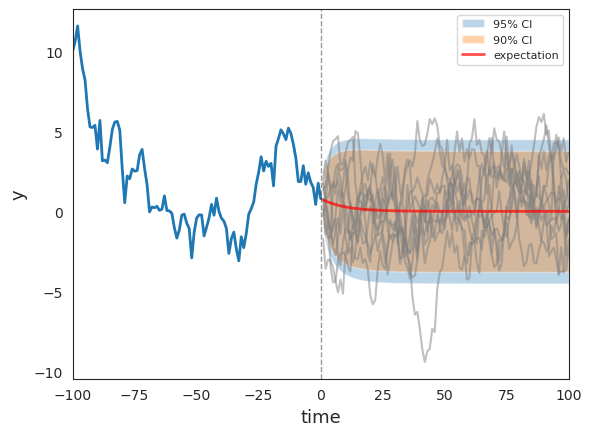
Fig. 20.1 Initial and predictive future paths#
As functions of forecast horizon, the coverage intervals have shapes like those described in Permanent Income II: LQ Techniques
20.3. Predictive Distributions of Path Properties#
Wecker [Wecker, 1979] proposed using simulation techniques to characterize the predictive distribution of some statistics that are non-linear functions of \(y\).
He called these functions “path properties” to contrast them with properties of single data points.
He studied two special prospective path properties of a given series \(\{y_t\}\).
The first was time until the next turning point.
he defined a “turning point” to be the date of the second of two successive declines in \(y\).
For example, if \(y_t(\omega)< y_{t-1}(\omega)< y_{t-2}(\omega)\), then period \(t\) is a turning point.
To examine the time until the next turning point, let \(Z\) be an indicator process
Here \(\omega \in \Omega\) is a sequence of events, and \(Y_t: \Omega \rightarrow \mathbb{R}\) gives \(y_t\) according to \(\omega\) and the AR(1) process.
By Wecker’s definition, period \(t\) is a turning point, and \(Y_{t-2}(\omega) \geq Y_{t-3}(\omega)\) excludes the possibility that period \(t-1\) is a turning point.
Then the random variable time until the next turning point is defined as the following stopping time with respect to \(Z\):
In the following code, we name this statistic time until the next recession to distinguish it from another concept of turning point.
Moreover, the statistic time until the next severe recession is defined in a similar way, except the decline between periods is greater than \(0.02\).
Wecker [Wecker, 1979] also studied the minimum value of \(Y\) over the next 8 quarters, which can be defined as the random variable
It is interesting to study yet another possible concept of a turning point.
Thus, let
Define a positive turning point today or tomorrow statistic as
This is designed to express the event
“after one or two decrease(s), \(Y\) will grow for two consecutive quarters”
The negative turning point today or tomorrow \(N_t\) is defined in the same way.
Following [Wecker, 1979], we can use simulations to calculate probabilities of \(P_t\) and \(N_t\) for each period \(t\).
However, in the following code, we only use \(T_{t+1}(\omega)=1\) to determine \(P_t(\omega)\) and \(N_t(\omega)\), because we only want to find the first positive turning point.
20.4. A Wecker-Like Algorithm#
The procedure consists of the following steps:
index a sample path by \(\omega_i\)
from a given date \(t\), simulate \(I\) sample paths of length \(N\)
for each path \(\omega_i\), compute the associated value of \(W_t(\omega_i), W_{t+1}(\omega_i), \dots , W_{t+N}\)
consider the sets \(\{W_t(\omega_i)\}^{I}_{i=1}, \ \{W_{t+1}(\omega_i)\}^{I}_{i=1}, \ \dots, \ \{W_{t+N}(\omega_i)\}^{I}_{i=1}\) as samples from the predictive distributions \(f(W_{t+1} \mid y_t, y_{t-1}, \dots , y_0)\), \(f(W_{t+2} \mid y_t, y_{t-1}, \dots , y_0)\), \(\dots\), \(f(W_{t+N} \mid y_t, y_{t-1}, \dots , y_0)\).
20.5. Using Simulations to Approximate a Posterior Distribution#
The next code cells use numpyro to compute the time \(t\) posterior distribution of \(\rho, \sigma\).
We construct this posterior just as in Posterior Distributions for AR(1) Parameters, to which we refer for a detailed discussion.
As there, in defining the likelihood function we condition on the initial value \(y_0\).
This is the conditioning assumption of Posterior Distributions for AR(1) Parameters, and it is the appropriate choice here because our initial path starts from an atypical value \(y_0 = 10\).
def draw_from_posterior(data, size=10000, dis_plot=True, key=key):
    """Draw a sample of the given size from the posterior distribution."""

    def model(data):
        # Start with priors
        ρ = numpyro.sample('ρ', dist.Uniform(-1, 1))  # Assume stable ρ
        σ = numpyro.sample('σ', dist.HalfNormal(jnp.sqrt(10)))

        # Expected value of y at the next period (ρ * y), conditioning on y_0
        yhat = ρ * data[:-1]

        # Likelihood of the actual realization
        numpyro.sample('y_obs', dist.Normal(yhat, σ), obs=data[1:])

    # Compute posterior distribution of parameters
    nuts_kernel = NUTS(model)

    # Define MCMC class to compute the posteriors
    mcmc = MCMC(
        nuts_kernel,
        num_warmup=5000,
        num_samples=size,
        num_chains=4,  # plot 4 chains in the trace
        progress_bar=False,
        chain_method='vectorized'
    )

    # Run MCMC
    mcmc.run(key, data=data)

    # Get posterior samples
    post_sample = {
        'ρ': mcmc.get_samples()['ρ'],
        'σ': mcmc.get_samples()['σ'],
    }

    # Plot posterior distributions and trace plots
    if dis_plot:
        plot_data = az.from_numpyro(posterior=mcmc)
        az.plot_trace_dist(plot_data, var_names=['ρ', 'σ'])

    return post_sample

post_samples = draw_from_posterior(initial_path)
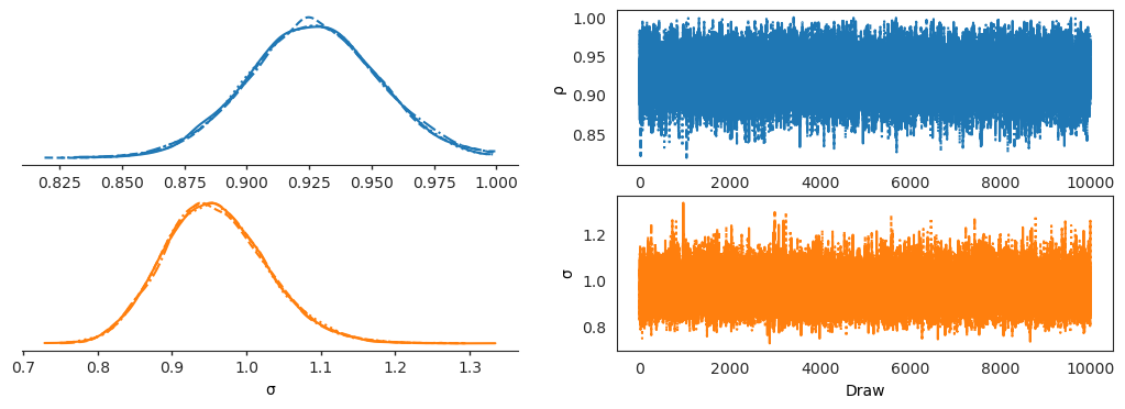
Fig. 20.2 Posterior and trace plots#
The graphs above portray posterior distributions and trace plots. The posterior distributions (left column) show the marginal distributions of the parameters after observing the data, while the trace plots (right column) help diagnose MCMC convergence by showing how the sampler explored the parameter space over iterations.
20.6. Calculating Sample Path Statistics#
Our next step is to prepare Python code to compute our sample path statistics.
These statistics were originally defined as random variables with respect to \(\omega\), but here we use \(\{Y_t\}\) as the argument because \(\omega\) is implicit.
These two kinds of definitions are equivalent because \(\omega\) determines path statistics only through \(\{Y_t\}\).
Moreover, we ignore all equality in the definitions, as equality occurs with zero probability for continuous random variables.
@jax.jit
def compute_path_statistics(initial_path, future_path):
    """Compute path statistics for the AR(1) process."""
    # Prepend the last three observed values so we can identify a turn at t=0
    y = jnp.concatenate([initial_path[-3:], future_path])
    n = y.shape[0]

    def step(carry, i):
        # identify recession
        rec_cond = (y[i] < y[i-1]) & (y[i-1] < y[i-2]) & (y[i-2] > y[i-3])
        # identify severe recession
        sev_cond = (
            (y[i] - y[i-1] < -0.02) & (y[i-1] - y[i-2] < -0.02) & (y[i-2] > y[i-3])
            )

        # identify positive turning point
        up_cond = (
            (y[i-2] > y[i-1]) & (y[i-1] > y[i]) & (y[i] < y[i+1]) & (y[i+1] < y[i+2])
        )

        # identify negative turning point
        down_cond = (
            (y[i-2] < y[i-1]) & (y[i-1] < y[i]) & (y[i] > y[i+1]) & (y[i+1] > y[i+2])
        )

        # Convert to int
        rec = jnp.where(rec_cond, 1, 0)
        sev = jnp.where(sev_cond, 1, 0)
        up = jnp.where(up_cond, 1, 0)
        down = jnp.where(down_cond, 1, 0)
        return carry, (rec, sev, up, down)

    _, (rec_seq, sev_seq, up_seq, down_seq) = lax.scan(step, None, jnp.arange(3, n-2))

    # Get the time until the first recession
    next_recession = jnp.where(
        jnp.any(rec_seq == 1), jnp.argmax(rec_seq == 1) + 1, len(y)
    )
    next_severe_recession = jnp.where(
        jnp.any(sev_seq == 1), jnp.argmax(sev_seq == 1) + 1, len(y)
    )

    # Minimum value in the next 8 periods
    min_val_8q = jnp.min(future_path[:8])

    # Get the time until the first turning point
    next_up_turn = jnp.where(
        jnp.any(up_seq == 1),
        jnp.maximum(jnp.argmax(up_seq == 1), 1), # Exclude 0 return
        len(y)
    )
    next_down_turn = jnp.where(
        jnp.any(down_seq == 1),
        jnp.maximum(jnp.argmax(down_seq == 1), 1),
        len(y)
    )
    path_stats = (
        next_recession, next_severe_recession, min_val_8q,
        next_up_turn, next_down_turn
        )
    return path_stats
The following function creates visualizations of the path statistics in a subplot grid.
def plot_path_stats(next_recession, next_severe_recession, min_val_8q,
                    next_up_turn, next_down_turn, ax, label=None):
    """Plot the path statistics in subplots(3,2)"""
    # ax[0, 0] is for paths of y
    sns.histplot(next_recession, kde=True, stat='density', ax=ax[0, 1],
                 alpha=.8, label=label)
    ax[0, 1].set_xlabel("time until the next recession", fontsize=13)

    sns.histplot(next_severe_recession, kde=True, stat='density', ax=ax[1, 0],
                 alpha=.8, label=label)
    ax[1, 0].set_xlabel("time until the next severe recession", fontsize=13)

    sns.histplot(min_val_8q, kde=True, stat='density', ax=ax[1, 1],
                 alpha=.8, label=label)
    ax[1, 1].set_xlabel("minimum value in next 8 periods", fontsize=13)

    sns.histplot(next_up_turn, kde=True, stat='density', ax=ax[2, 0],
                 alpha=.8, label=label)
    ax[2, 0].set_xlabel("time until the next positive turn", fontsize=13)

    sns.histplot(next_down_turn, kde=True, stat='density', ax=ax[2, 1],
                 alpha=.8, label=label)
    ax[2, 1].set_xlabel("time until the next negative turn", fontsize=13)
20.7. Original Wecker Method#
Now we apply Wecker’s original method by simulating future paths and compute predictive distributions, conditioning on the true parameters associated with the data-generating model.
def plot_Wecker(ar1: AR1, initial_path, ax, N=1000, label='true parameters'):
    """
    Plot the predictive distributions from "pure" Wecker's method.

    Parameters
    ----------
    ar1 : AR1
        An AR1 named tuple containing the process parameters (ρ, σ, T0, T1).
    initial_path : array-like
        The initial observed path of the AR(1) process.
    N : int
        Number of future sample paths to simulate for predictive distributions.
    label : str
        Legend label for the plotted distributions.
    """
    # Plot simulated initial and future paths
    y_T0 = initial_path[-1]
    future_path = AR1_simulate_future(ar1, y_T0, N=N)
    plot_path(ar1, initial_path, future_path, ax[0, 0])

    next_reces = jnp.zeros(N)
    severe_rec = jnp.zeros(N)
    min_val_8q = jnp.zeros(N)
    next_up_turn = jnp.zeros(N)
    next_down_turn = jnp.zeros(N)

    # Simulate future paths and compute statistics
    for n in range(N):
        future_temp = future_path[n, :]
        (next_reces_val, severe_rec_val, min_val_8q_val,
        next_up_turn_val, next_down_turn_val
         ) = compute_path_statistics(initial_path, future_temp)

        next_reces = next_reces.at[n].set(next_reces_val)
        severe_rec = severe_rec.at[n].set(severe_rec_val)
        min_val_8q = min_val_8q.at[n].set(min_val_8q_val)
        next_up_turn = next_up_turn.at[n].set(next_up_turn_val)
        next_down_turn = next_down_turn.at[n].set(next_down_turn_val)

    # Plot path statistics
    plot_path_stats(next_reces, severe_rec, min_val_8q,
                    next_up_turn, next_down_turn, ax, label=label)


fig, ax = plt.subplots(3, 2, figsize=(15, 12))
plot_Wecker(ar1, initial_path, ax)
plt.show()
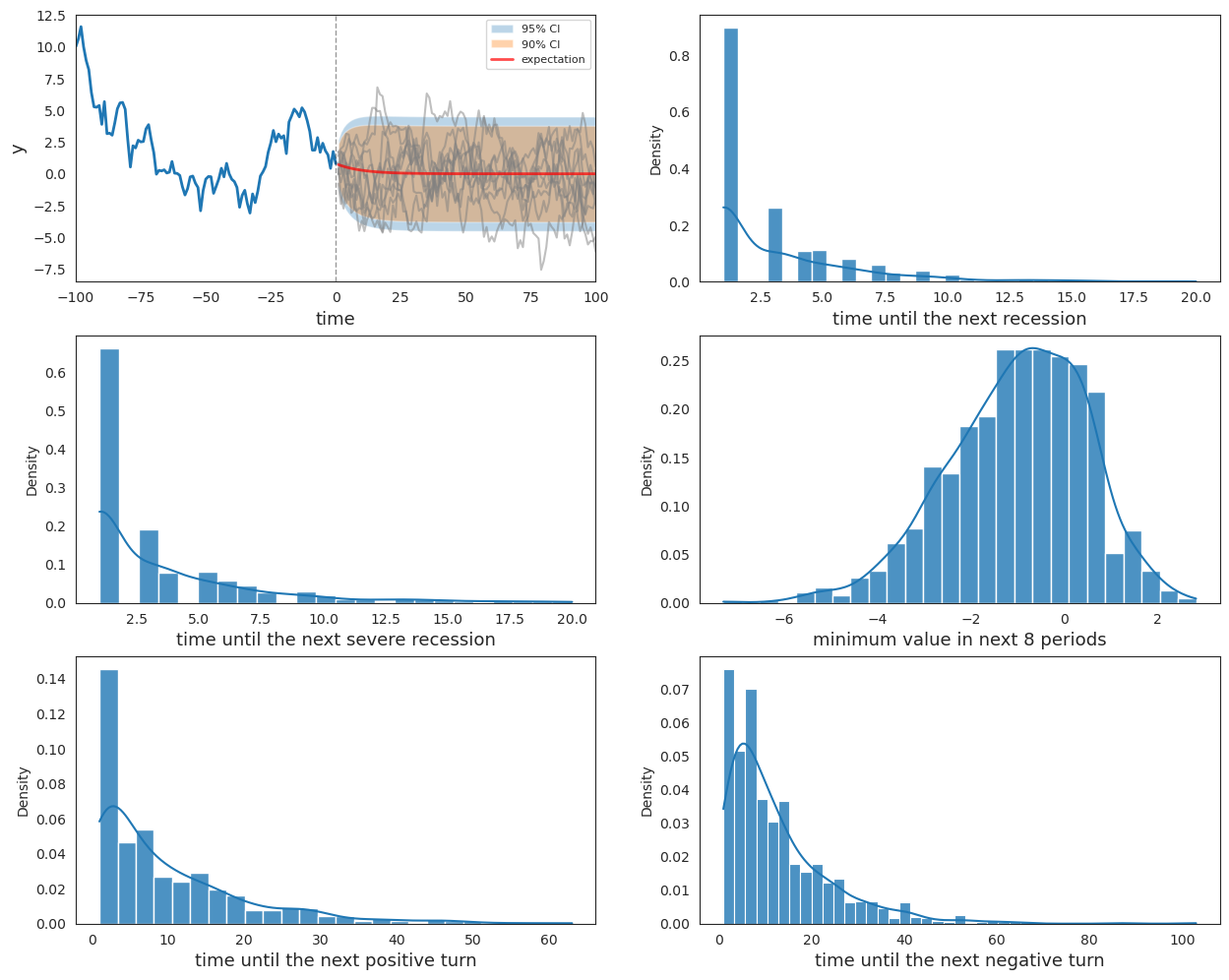
Fig. 20.3 Distributions from Wecker’s method#
Apart from the top-left panel, which repeats the initial path and coverage intervals, each panel shows the predictive distribution of one sample path statistic.
These are computed by simulating many future paths with the parameters held fixed at their true values.
The distributions therefore reflect only the uncertainty that comes from future shocks.
20.8. Extended Wecker Method#
Now we apply our “extended” Wecker method based on predictive densities of \(y\) defined by (20.4) that acknowledge posterior uncertainty in the parameters \(\rho, \sigma\).
To approximate the integration on the right side of (20.4), we repeatedly draw parameters from the joint posterior distribution each time we simulate a sequence of future values from model (20.1).
def plot_extended_Wecker(
    ar1: AR1, post_samples, initial_path, ax, N=1000,
    label='sampling from posterior'
    ):
    """Plot the extended Wecker's predictive distribution"""
    y0, T1 = ar1.y0, ar1.T1
    y_T0 = initial_path[-1]

    # Select a parameter sample
    index = random.choice(
        key, jnp.arange(len(post_samples['ρ'])), (N,), replace=False
        )
    ρ_sample = post_samples['ρ'][index]
    σ_sample = post_samples['σ'][index]

    # Compute path statistics
    next_reces = jnp.zeros(N)
    severe_rec = jnp.zeros(N)
    min_val_8q = jnp.zeros(N)
    next_up_turn = jnp.zeros(N)
    next_down_turn = jnp.zeros(N)

    subkeys = random.split(key, num=N)

    # Simulate one future path per posterior draw
    future_paths = []
    for n in range(N):
        ar1_n = AR1(ρ=ρ_sample[n], σ=σ_sample[n], y0=y0, T1=T1)
        future_temp = AR1_simulate_future(
            ar1_n, y_T0, N=1, key=subkeys[n]
            ).reshape(-1)
        future_paths.append(future_temp)
        (next_reces_val, severe_rec_val, min_val_8q_val,
        next_up_turn_val, next_down_turn_val
         ) = compute_path_statistics(initial_path, future_temp)

        next_reces = next_reces.at[n].set(next_reces_val)
        severe_rec = severe_rec.at[n].set(severe_rec_val)
        min_val_8q = min_val_8q.at[n].set(min_val_8q_val)
        next_up_turn = next_up_turn.at[n].set(next_up_turn_val)
        next_down_turn = next_down_turn.at[n].set(next_down_turn_val)

    # Plot the initial path and the future paths drawn from the posterior
    future_paths = jnp.stack(future_paths)
    plot_path(ar1, initial_path, future_paths, ax[0, 0])

    # Plot path statistics
    plot_path_stats(next_reces, severe_rec, min_val_8q,
                    next_up_turn, next_down_turn, ax, label=label)

fig, ax = plt.subplots(3, 2, figsize=(12, 15))
plot_extended_Wecker(ar1, post_samples, initial_path, ax)
plt.show()
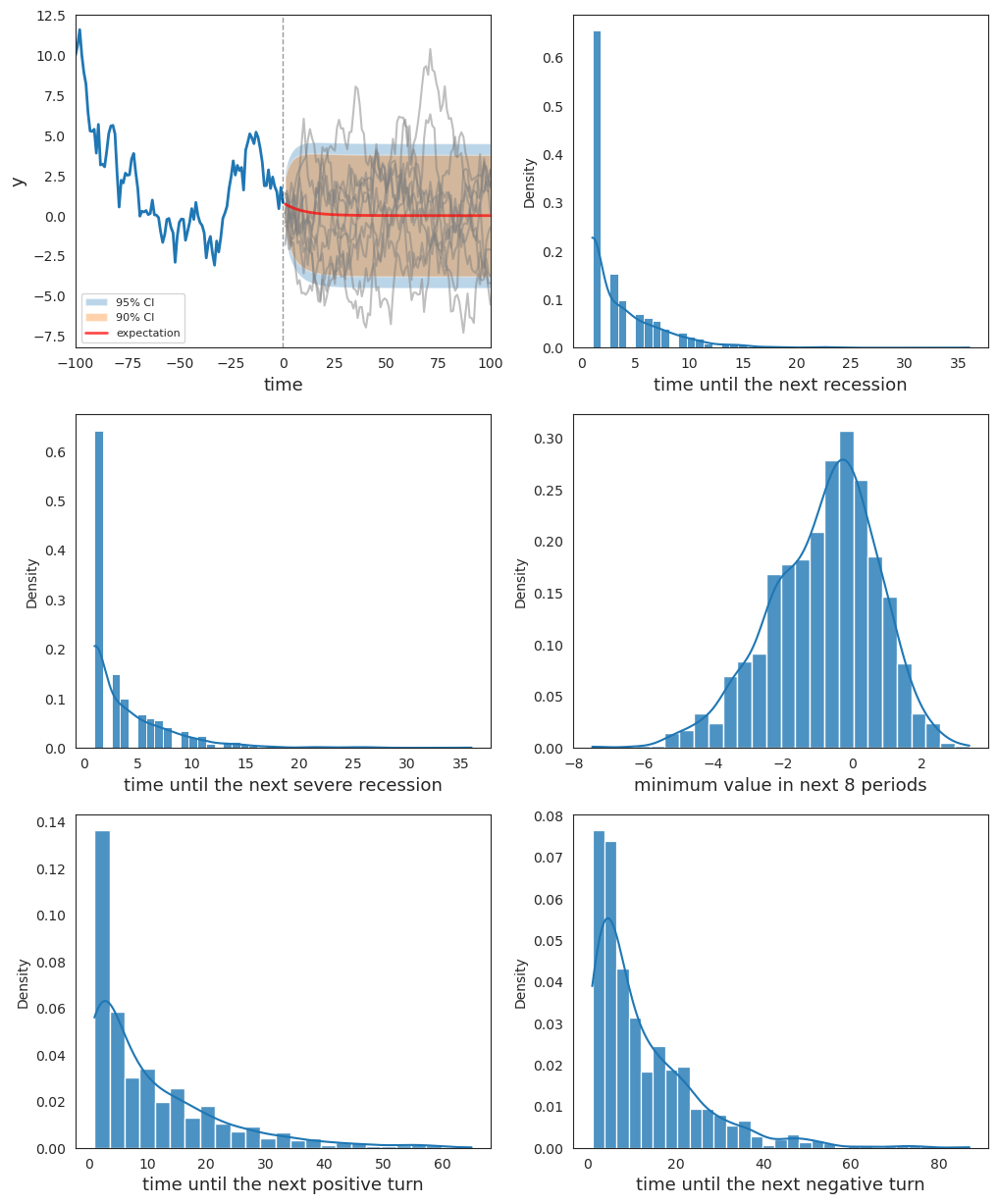
Fig. 20.4 Distributions from extended Wecker’s method#
The panels show the same statistics, but now each future path is simulated with parameters drawn from the posterior.
These distributions therefore combine two sources of uncertainty: randomness in future shocks and our uncertainty about \((\rho, \sigma)\).
20.9. Comparison#
Finally, we plot both the original Wecker method and the extended method with parameter values drawn from the posterior together to compare the differences that emerge from pretending to know parameter values when they are actually uncertain.
fig, ax = plt.subplots(3, 2, figsize=(12, 15))
plot_Wecker(ar1, initial_path, ax)
ax[0, 0].clear()
plot_extended_Wecker(ar1, post_samples, initial_path, ax)
ax[0, 1].legend(fontsize=10)
plt.show()
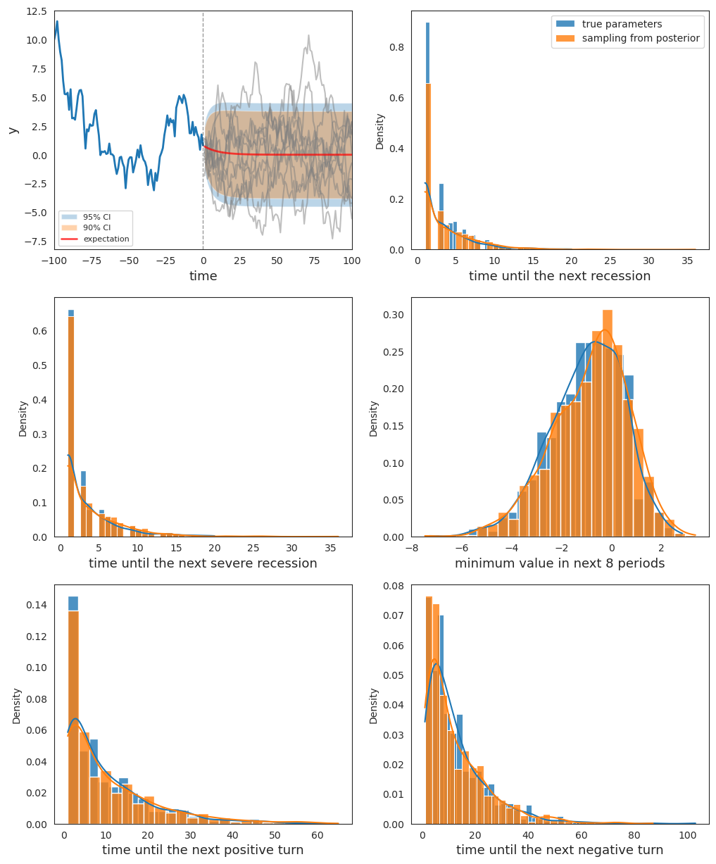
Fig. 20.5 Comparison of the two methods#
The two sets of predictive distributions reveal the cost of pretending that we know the parameters.
The extended Wecker method draws \((\rho, \sigma)\) from their posterior each time it simulates a future path.
It therefore layers parameter uncertainty on top of the shock uncertainty already present in the original method.
As a result, its predictive distributions are more dispersed than those computed with the parameters fixed at their true values.
20.10. Conclusion#
This lecture combined two tools to forecast nonlinear functions of the future path of an AR(1) process.
Wecker’s simulation method let us approximate predictive distributions of sample path statistics, such as the time until the next turning point.
A Bayesian posterior over \((\rho, \sigma)\), computed as in Posterior Distributions for AR(1) Parameters, let us also account for our uncertainty about the parameters that govern the process.
Putting these together, the extended Wecker method produces predictive distributions that reflect both sources of uncertainty identified at the outset.
Ignoring parameter uncertainty, as the original Wecker method does, yields tighter distributions that overstate how much we really know about these future statistics.