15. Introduction to Artificial Neural Networks#
GPU
This lecture was built using a machine with access to a GPU — although it will also run without one.
Google Colab has a free tier with GPUs that you can access as follows:
Click on the “play” icon top right
Select Colab
Set the runtime environment to include a GPU
In addition to what’s included in base Anaconda, we need to install the following packages
!pip install -U kaleido plotly
!conda install -y -c plotly plotly-orca

# kaleido needs chrome to build images
import kaleido
kaleido.get_chrome_sync()
Note
If you are running this on Google Colab the above cell will
present an error. This is because Google Colab doesn’t use Anaconda to manage
the Python packages. However this lecture will still execute as Google Colab
has plotly installed.
We also need to install JAX to run this lecture
!pip install --upgrade jax
import jax
print(f"JAX backend: {jax.devices()[0].platform}") # to check that gpu is activated in environment
JAX backend: gpu
15.1. Overview#
Substantial parts of machine learning and artificial intelligence are about
approximating an unknown function with a known function
estimating the known function from a set of data on the left- and right-hand variables
This lecture describes the structure of a plain vanilla artificial neural network (ANN) of a type that is widely used to approximate a function \(f\) that maps \(x\) in a space \(X\) into \(y\) in a space \(Y\).
To introduce elementary concepts, we study an example in which \(x\) and \(y\) are scalars.
We’ll describe the following concepts that are brick and mortar for neural networks:
a neuron
an activation function
a network of neurons
A neural network as a composition of functions
back-propagation and its relationship to the chain rule of differential calculus
15.2. A Deep (but not Wide) Artificial Neural Network#
We describe a “deep” neural network of “width” one.
Deep means that the network composes a large number of functions organized into nodes of a graph.
Width refers to the number of right hand side variables on the right hand side of the function being approximated.
Setting “width” to one means that the network composes just univariate functions.
Let \(x \in \mathbb{R}\) be a scalar and \(y \in \mathbb{R}\) be another scalar.
We assume that \(y\) is a nonlinear function of \(x\):
We want to approximate \(f(x)\) with another function that we define recursively.
For a network of depth \(N \geq 1\), each layer \(i =1, \ldots N\) consists of
an input \(x_i\)
an affine function \(w_i x_i + bI\), where \(w_i\) is a scalar weight placed on the input \(x_i\) and \(b_i\) is a scalar bias
an activation function \(h_i\) that takes \((w_i x_i + b_i)\) as an argument and produces an output \(x_{i+1}\)
An example of an activation function \(h\) is the sigmoid function
Another popular activation function is the rectified linear unit (ReLU) function
Yet another activation function is the identity function
As activation functions below, we’ll use the sigmoid function for layers \(1\) to \(N-1\) and the identity function for layer \(N\).
To approximate a function \(f(x)\) we construct \(\hat f(x)\) by proceeding as follows.
Let
We construct \(\hat f\) by iterating on compositions of functions \(h_i \circ l_i\):
If \(N >1\), we call the right side a “deep” neural net.
The larger is the integer \(N\), the “deeper” is the neural net.
Evidently, if we know the parameters \(\{w_i, b_i\}_{i=1}^N\), then we can compute \(\hat f(x)\) for a given \(x = \tilde x\) by iterating on the recursion
starting from \(x_1 = \tilde x\).
The value of \(x_{N+1}\) that emerges from this iterative scheme equals \(\hat f(\tilde x)\).
15.3. Calibrating Parameters#
We now consider a neural network like the one describe above with width 1, depth \(N\), and activation functions \(h_{i}\) for \(1\leqslant i\leqslant N\) that map \(\mathbb{R}\) into itself.
Let \(\left\{ \left(w_{i},b_{i}\right)\right\} _{i=1}^{N}\) denote a sequence of weights and biases.
As mentioned above, for a given input \(x_{1}\), our approximating function \(\hat f\) evaluated at \(x_1\) equals the “output” \(x_{N+1}\) from our network that can be computed by iterating on \(x_{i+1}=h_{i}\left(w_{i}x_{i}+b_{i}\right)\).
For a given prediction \(\hat{y} (x) \) and target \(y= f(x)\), consider the loss function
This criterion is a function of the parameters \(\left\{ \left(w_{i},b_{i}\right)\right\} _{i=1}^{N}\) and the point \(x\).
We’re interested in solving the following problem:
where \(\mu(x)\) is some measure of points \(x \in \mathbb{R}\) over which we want a good approximation \(\hat f(x)\) to \(f(x)\).
Stack weights and biases into a vector of parameters \(p\):
Applying a “poor man’s version” of a stochastic gradient descent algorithm for finding a zero of a function leads to the following update rule for parameters:
where \(\frac{d {\mathcal L}}{dx_{N+1}}=-\left(x_{N+1}-y\right)\) and \(\alpha > 0 \) is a step size.
(See this and this to gather insights about how stochastic gradient descent relates to Newton’s method.)
To implement one step of this parameter update rule, we want the vector of derivatives \(\frac{dx_{N+1}}{dp_k}\).
In the neural network literature, this step is accomplished by what is known as back propagation.
15.4. Back Propagation and the Chain Rule#
Thanks to properties of
the chain and product rules for differentiation from differential calculus, and
lower triangular matrices
back propagation can actually be accomplished in one step by
inverting a lower triangular matrix, and
matrix multiplication
(This idea is from the last 7 minutes of this great youtube video by MIT’s Alan Edelman)
Here goes.
Define the derivative of \(h(z)\) with respect to \(z\) evaluated at \(z = z_i\) as \(\delta_i\):
or
Repeated application of the chain rule and product rule to our recursion (15.1) allows us to obtain:
After imposing \(dx_{1}=0\), we get the following system of equations:
or
which implies that
which in turn implies
We can then solve the above problem by applying our update for \(p\) multiple times for a collection of input-output pairs \(\left\{ \left(x_{1}^{i},y^{i}\right)\right\} _{i=1}^{M}\) that we’ll call our “training set”.
15.5. Training Set#
Choosing a training set amounts to a choice of measure \(\mu\) in the above formulation of our function approximation problem as a minimization problem.
In this spirit, we shall use a uniform grid of, say, 50 or 200 points.
There are many possible approaches to the minimization problem posed above:
batch gradient descent in which you use an average gradient over the training set
stochastic gradient descent in which you sample points randomly and use individual gradients
something in-between (so-called “mini-batch gradient descent”)
The update rule (15.2) described above amounts to a stochastic gradient descent algorithm.
from IPython.display import Image
import jax.numpy as jnp
from jax import grad, jit, jacfwd, vmap
from jax import random
import jax
import plotly.graph_objects as go
# A helper function to randomly initialize weights and biases
# for a dense neural network layer
def random_layer_params(m, n, key, scale=1.):
    w_key, b_key = random.split(key)
    return scale * random.normal(w_key, (n, m)), scale * random.normal(b_key, (n,))

# Initialize all layers for a fully-connected neural network with sizes "sizes"
def init_network_params(sizes, key):
    keys = random.split(key, len(sizes))
    return [random_layer_params(m, n, k) for m, n, k in zip(sizes[:-1], sizes[1:], keys)]
def compute_xδw_seq(params, x):
    # Initialize arrays
    δ = jnp.zeros(len(params))
    xs = jnp.zeros(len(params) + 1)
    ws = jnp.zeros(len(params))
    bs = jnp.zeros(len(params))

    h = jax.nn.sigmoid

    xs = xs.at[0].set(x)
    for i, (w, b) in enumerate(params[:-1]):
        output = w * xs[i] + b
        activation = h(output[0, 0])

        # Store elements
        δ = δ.at[i].set(grad(h)(output[0, 0]))
        ws = ws.at[i].set(w[0, 0])
        bs = bs.at[i].set(b[0])
        xs = xs.at[i+1].set(activation)

    final_w, final_b = params[-1]
    preds = final_w * xs[-2] + final_b

    # Store elements
    δ = δ.at[-1].set(1.)
    ws = ws.at[-1].set(final_w[0, 0])
    bs = bs.at[-1].set(final_b[0])
    xs = xs.at[-1].set(preds[0, 0])

    return xs, δ, ws, bs


def loss(params, x, y):
    xs, δ, ws, bs = compute_xδw_seq(params, x)
    preds = xs[-1]

    return 1 / 2 * (y - preds) ** 2
# Parameters
N = 3  # Number of layers
layer_sizes = [1, ] * (N + 1)
param_scale = 0.1
step_size = 0.01
params = init_network_params(layer_sizes, random.PRNGKey(1))
x = 5
y = 3
xs, δ, ws, bs = compute_xδw_seq(params, x)
dxs_ad = jacfwd(lambda params, x: compute_xδw_seq(params, x)[0], argnums=0)(params, x)
dxs_ad_mat = jnp.block([dx.reshape((-1, 1)) for dx_tuple in dxs_ad for dx in dx_tuple ])[1:]
jnp.block([[δ * xs[:-1]], [δ]])
Array([[1.0165801 , 0.06087969, 0.09382247],
       [0.20331602, 0.08501981, 1.        ]], dtype=float32)
L = jnp.diag(δ * ws, k=-1)
L = L[1:, 1:]

D = jax.scipy.linalg.block_diag(*[row.reshape((1, 2)) for row in jnp.block([[δ * xs[:-1]], [δ]]).T])

dxs_la = jax.scipy.linalg.solve_triangular(jnp.eye(N) - L, D, lower=True)
# Check that the `dx` generated by the linear algebra method
# are the same as the ones generated using automatic differentiation
jnp.max(jnp.abs(dxs_ad_mat - dxs_la))
Array(0., dtype=float32)
grad_loss_ad = jnp.block([dx.reshape((-1, 1)) for dx_tuple in grad(loss)(params, x, y) for dx in dx_tuple ])
# Check that the gradient of the loss is the same for both approaches
jnp.max(jnp.abs(-(y - xs[-1]) * dxs_la[-1] - grad_loss_ad))
Array(5.9604645e-08, dtype=float32)
@jit
def update_ad(params, x, y):
    grads = grad(loss)(params, x, y)
    return [(w - step_size * dw, b - step_size * db)
          for (w, b), (dw, db) in zip(params, grads)]

@jit
def update_la(params, x, y):
    xs, δ, ws, bs = compute_xδw_seq(params, x)
    N = len(params)
    L = jnp.diag(δ * ws, k=-1)
    L = L[1:, 1:]

    D = jax.scipy.linalg.block_diag(*[row.reshape((1, 2)) for row in jnp.block([[δ * xs[:-1]], [δ]]).T])

    dxs_la = jax.scipy.linalg.solve_triangular(jnp.eye(N) - L, D, lower=True)

    grads = -(y - xs[-1]) * dxs_la[-1]

    return [(w - step_size * dw, b - step_size * db)
            for (w, b), (dw, db) in zip(params, grads.reshape((-1, 2)))]
# Check that both updates are the same
update_la(params, x, y)
[(Array([[-0.00826643]], dtype=float32), Array([0.94700736], dtype=float32)),
 (Array([[-2.0638916]], dtype=float32), Array([-0.7872697], dtype=float32)),
 (Array([[1.6248171]], dtype=float32), Array([1.5765371], dtype=float32))]
update_ad(params, x, y)
[(Array([[-0.00826644]], dtype=float32), Array([0.94700736], dtype=float32)),
 (Array([[-2.0638916]], dtype=float32), Array([-0.7872697], dtype=float32)),
 (Array([[1.6248171]], dtype=float32), Array([1.5765371], dtype=float32))]
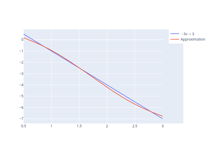
15.6. Example 1#
Consider the function
on \(\left[0.5,3\right]\).
We use a uniform grid of 200 points and update the parameters for each point on the grid 300 times.
\(h_{i}\) is the sigmoid activation function for all layers except the final one for which we use the identity function and \(N=3\).
Weights are initialized randomly.
def f(x):
    return -3 * x + 2

M = 200
grid = jnp.linspace(0.5, 3, num=M)
f_val = f(grid)
indices = jnp.arange(M)
key = random.PRNGKey(0)

def train(params, grid, f_val, key, num_epochs=300):
    for epoch in range(num_epochs):
        key, _ = random.split(key)
        random_permutation = random.permutation(random.PRNGKey(1), indices)
        for x, y in zip(grid[random_permutation], f_val[random_permutation]):
            params = update_la(params, x, y)

    return params
# Parameters
N = 3  # Number of layers
layer_sizes = [1, ] * (N + 1)
params_ex1 = init_network_params(layer_sizes, key)
%%time
params_ex1 = train(params_ex1, grid, f_val, key, num_epochs=500)
CPU times: user 18 s, sys: 4.52 s, total: 22.5 s
Wall time: 15.5 s
predictions = vmap(compute_xδw_seq, in_axes=(None, 0))(params_ex1, grid)[0][:, -1]
fig = go.Figure()
fig.add_trace(go.Scatter(x=grid, y=f_val, name=r'$-3x+2$'))
fig.add_trace(go.Scatter(x=grid, y=predictions, name='Approximation'))

# Export to PNG file
Image(fig.to_image(format="png"))
# fig.show() will provide interactive plot when running
# notebook locally
15.7. How Deep?#
It is fun to think about how deepening the neural net for the above example affects the quality of approximation
If the network is too deep, you’ll run into the vanishing gradient problem
Other parameters such as the step size and the number of epochs can be as important or more important than the number of layers in the situation considered in this lecture.
Indeed, since \(f\) is a linear function of \(x\), a one-layer network with the identity map as an activation would probably work best.
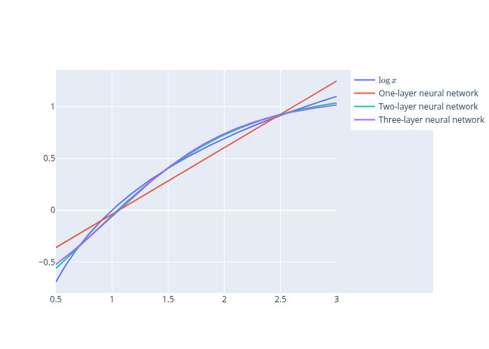
15.8. Example 2#
We use the same setup as for the previous example with
def f(x):
    return jnp.log(x)

grid = jnp.linspace(0.5, 3, num=M)
f_val = f(grid)
# Parameters
N = 1  # Number of layers
layer_sizes = [1, ] * (N + 1)
params_ex2_1 = init_network_params(layer_sizes, key)
# Parameters
N = 2  # Number of layers
layer_sizes = [1, ] * (N + 1)
params_ex2_2 = init_network_params(layer_sizes, key)
# Parameters
N = 3  # Number of layers
layer_sizes = [1, ] * (N + 1)
params_ex2_3 = init_network_params(layer_sizes, key)
params_ex2_1 = train(params_ex2_1, grid, f_val, key, num_epochs=300)
params_ex2_2 = train(params_ex2_2, grid, f_val, key, num_epochs=300)
params_ex2_3 = train(params_ex2_3, grid, f_val, key, num_epochs=300)
predictions_1 = vmap(compute_xδw_seq, in_axes=(None, 0))(params_ex2_1, grid)[0][:, -1]
predictions_2 = vmap(compute_xδw_seq, in_axes=(None, 0))(params_ex2_2, grid)[0][:, -1]
predictions_3 = vmap(compute_xδw_seq, in_axes=(None, 0))(params_ex2_3, grid)[0][:, -1]
fig = go.Figure()
fig.add_trace(go.Scatter(x=grid, y=f_val, name=r'$\log{x}$'))
fig.add_trace(go.Scatter(x=grid, y=predictions_1, name='One-layer neural network'))
fig.add_trace(go.Scatter(x=grid, y=predictions_2, name='Two-layer neural network'))
fig.add_trace(go.Scatter(x=grid, y=predictions_3, name='Three-layer neural network'))

# Export to PNG file
Image(fig.to_image(format="png"))
# fig.show() will provide interactive plot when running
# notebook locally