23. Information Projections#
23.1. Overview#
In Euclidean geometry, the projection of a point onto a set is the point of the set that is closest to it.
When the set is a line or a plane, the projection is unique, the segment joining the point to its projection meets the set at a right angle, and the Pythagorean theorem holds.
This lecture describes analogous results for probability distributions, with the Kullback–Leibler (KL) divergence in place of squared distance.
A distribution has two kinds of projection onto a set \(\mathcal{S}\) of distributions, because KL divergence is not symmetric:
the e-projection of \(q\) onto \(\mathcal{S}\) is the \(p \in \mathcal{S}\) that minimizes \(D_{KL}(p \| q)\), so the distribution being projected is the second argument; and
the m-projection of \(p\) onto \(\mathcal{S}\) is the \(q \in \mathcal{S}\) that minimizes \(D_{KL}(p \| q)\), so the distribution being projected is the first argument.
Two kinds of “flat” sets of distributions serve as lines and planes:
linear families, such as the set of distributions that give a statistic a prescribed mean; a linear family contains every mixture \((1 - a) p_0 + a p_1\) of two of its members, for every real \(a\) for which the mixture is a probability distribution; and
exponential families, described in Exponential Family and Maximum Entropy; an exponential family contains every normalized geometric mixture of two of its members, for every real \(a\) for which the geometric mixture can be normalized.
The e-projection onto a linear family and the m-projection onto an exponential family are unique, and each satisfies a Pythagorean theorem.
The two projections have simple forms:
the e-projection of \(q\) onto a linear family defined by moment conditions is an exponential tilt of \(q\), a distribution proportional to \(q(x) e^{\theta \cdot t(x)}\) for a vector \(\theta\) that satisfies the moment conditions; and
the m-projection of \(p\) onto an exponential family matches moments: it is the member of the family that gives the sufficient statistic the same means as \(p\) does.
These two facts organize several ideas that economists use:
maximum likelihood estimation, under correct specification and under misspecification (m-projections);
mutual information, which measures dependence between random variables (an m-projection);
maximum entropy, Sanov’s theorem, and large deviations (e-projections);
the worst-case models of robust control (e-projections);
the RAS method for updating input–output tables, and Sinkhorn’s algorithm for entropy-regularized optimal transport (repeated e-projections); and
the Chernoff information that governs error rates in tests based on likelihood ratios (an e-projection of two distributions at once).
The worst-case models of robust control and the solutions of the RAS and Sinkhorn problems are exponential tilts of the kind that attains the logit formula (22.12) of Exponential Family and Maximum Entropy.
This lecture builds on Exponential Family and Maximum Entropy and on Statistical Divergence Measures.
Csiszár [1975] developed the theory of e-projections, which he called I-projections.
Csiszár and Shields [2004] survey the theory and its statistical applications.
Nielsen [2018] is a short introduction to information projections, and Amari and Nagaoka [2000] treat them as part of information geometry.
We use the following imports.
import numpy as np
import matplotlib.pyplot as plt
from scipy import integrate
from scipy.optimize import brentq, linprog, minimize, minimize_scalar
from scipy.special import logsumexp, betaln, digamma
from scipy.stats import norm, poisson, chi2
import warnings
We write \(D(p \| q)\) for the KL divergence \(D_{KL}(p \| q)\) and, as in Exponential Family and Maximum Entropy, read it as “the divergence of \(p\) from \(q\).”
We write \(q_\theta\) for the members of an exponential family, because they usually appear in the second argument of \(D\).
Most of our examples use distributions on a finite set.
The functions below compute KL divergence, construct the exponential tilt that raises the probability of each outcome \(x\) in proportion to \(e^{\theta \cdot t(x)}\), and find the tilt that gives a scalar statistic a prescribed mean.
These generalize the functions of the same names in Exponential Family and Maximum Entropy: tilt also accepts vector-valued statistics, and match_mean accepts a bracket for its root finder.
def kl(p, q):
    """KL divergence of distributions (or arrays) p and q of equal shape."""
    p, q = np.ravel(p), np.ravel(q)
    if np.any(p < 0) or np.any(q < 0):
        raise ValueError("probabilities must be nonnegative")
    mask = p > 0                       # use the convention 0 log 0 = 0
    return np.sum(p[mask] * np.log(p[mask] / q[mask]))


def tilt(q, t, θ):
    """The distribution proportional to q(x) exp(θ · t(x)).

    t is either a vector of values t(x) or an array whose rows are t(x).
    """
    T = np.reshape(t, (len(q), -1))
    log_w = np.log(q) + T @ np.atleast_1d(θ)
    return np.exp(log_w - logsumexp(log_w))


def match_mean(q, t, c, bracket=(-50, 50)):
    """Find θ such that the tilt of q has E[t(X)] = c, for scalar t."""
    θ = brentq(lambda θ: tilt(q, t, θ) @ t - c, *bracket)
    return θ, tilt(q, t, θ)


rng = np.random.default_rng(1234)
23.2. A three-point identity#
Let \(p\), \(q\), and \(r\) be three probability distributions on a finite set, with \(q\) and \(r\) assigning positive probability to every outcome.
Expanding the definition of KL divergence gives the identity
The Euclidean analog is
The Euclidean cross term is an inner product of two displacements, and it vanishes when the segments from \(q\) to \(p\) and from \(q\) to \(r\) are perpendicular.
In (23.1), the cross term is an inner product of two displacements measured in different coordinates: \(p - q\) is a displacement in probabilities, and \(\log q - \log r\) is a displacement in log probabilities.
In the language of Exponential Family and Maximum Entropy, the distributions with full support on a finite set \(\{x_0, x_1, \ldots\}\) form an exponential family, whose expectation parameters are the probabilities \(p(x)\) and whose natural parameters are the log ratios \(\log(p(x)/p(x_0))\), for \(x \neq x_0\).
Probabilities are expectation parameters; log probabilities are, up to a normalization, natural parameters.
When the cross term vanishes, KL divergence satisfies a Pythagorean theorem,
We check (23.1) with randomly drawn distributions.
p, q, r = rng.dirichlet(np.ones(5), size=3)
lhs = kl(p, r)
rhs = kl(p, q) + kl(q, r) + (p - q) @ (np.log(q) - np.log(r))
print(f"D(p || r) = {lhs:.10f}")
print(f"right side = {rhs:.10f}")
D(p || r) = 0.4218836412
right side = 0.4218836412
The rest of this lecture is about sets of distributions on which the cross term vanishes.
We state and prove the theorems below for distributions on finite sets.
The identity (23.1), and everything we derive from it, also holds for densities, with integrals in place of sums, whenever the divergences are finite.
23.3. Two kinds of straight lines#
Two natural paths lead from a distribution \(p_0\) to a distribution \(p_1\).
The mixture path moves along a straight line in probabilities:
The exponential path moves along a straight line in log probabilities and then normalizes:
where \(F(a) = \log \sum_x p_0(x)^{1 - a} p_1(x)^a\).
Values of \(a\) in \([0, 1]\) trace out a path from \(p_0\) to \(p_1\); other values of \(a\) extend the path beyond its endpoints, the exponential path for every real \(a\) and the mixture path for as long as \(p_a\) stays nonnegative.
The exponential path is a one-parameter exponential family with sufficient statistic \(\log(p_1 / p_0)\) and natural parameter \(a\).
A geodesic is a geometry’s analog of a straight line.
Information geometers call these paths m-geodesics, for mixture, and e-geodesics, for exponential.
In the coordinates described after (23.1), an m-geodesic is a straight line in expectation parameters, and an e-geodesic is a straight line in natural parameters.
A set of distributions is m-flat if, whenever it contains \(p_0\) and \(p_1\), it contains \(p_a\) on the mixture path for every real \(a\) for which \(p_a\) is a probability distribution, not only for \(a \in [0, 1]\); it is e-flat if the same holds for exponential paths.
A set that contains the mixture segments with \(a \in [0, 1]\), but not necessarily the whole lines through its members, is merely convex in the ordinary sense.
The e-projection onto a closed convex set is still unique, but the Pythagorean identity (23.2) below weakens to the inequality \(D(p \| q) \geq D(p \| p^*) + D(p^* \| q)\) [Csiszár, 1975].
Two kinds of sets are the leading examples.
A linear family \(\mathcal{L} = \{ p : E_p[t(X)] = c \}\), the set of distributions that give a statistic \(t\) a prescribed mean, is m-flat, because if \(p_0\) and \(p_1\) satisfy \(E[t(X)] = c\), so does \((1 - a) p_0 + a p_1\) for every real \(a\).
An exponential family \(\mathcal{E} = \{ q_\theta : q_\theta(x) \propto h(x) \exp(\theta \cdot t(x)) \}\) is e-flat, because the logarithm of a normalized geometric mixture of \(q_{\theta_0}\) and \(q_{\theta_1}\) is \(\log h + ((1 - a) \theta_0 + a \theta_1) \cdot t\) plus a constant, for every real \(a\) for which the normalized geometric mixture exists.
A linear family is a straight line or plane in expectation parameters, the probabilities.
When \(h > 0\) everywhere, an exponential family is a straight line or plane in natural parameters, because \(\log(q_\theta(x) / q_\theta(x_0)) = \log(h(x)/h(x_0)) + \theta \cdot (t(x) - t(x_0))\) is an affine function of \(\theta\).
Distributions on three outcomes live in a triangle, the probability simplex, in which we can draw both kinds of sets.
The function below maps a distribution on three outcomes to a point in an equilateral triangle whose corners represent the three outcomes.
Each corner is the distribution that puts probability one on an outcome, the center is the uniform distribution, and the probability that a point \(p\) assigns to outcome \(x\) is proportional to the distance from \(p\) to the side opposite corner \(x\).
corners = np.array([[0.0, 0.0], [1.0, 0.0], [0.5, np.sqrt(3) / 2]])


def to_triangle(p):
    """Map distributions on three outcomes (rows of p) to the plane."""
    return np.atleast_2d(p) @ corners


def draw_simplex(ax, labels=("$x = 0$", "$x = 1$", "$x = 2$")):
    ax.plot(*np.vstack([corners, corners[0]]).T, color="0.6", lw=1)
    offsets = [(-0.07, -0.05), (0.02, -0.05), (-0.03, 0.03)]
    for corner, label, (dx, dy) in zip(corners, labels, offsets):
        ax.text(corner[0] + dx, corner[1] + dy, label)
    ax.set_aspect("equal")
    ax.axis("off")


def mixture_path(p0, p1, a):
    return (1 - a)[:, None] * p0 + a[:, None] * p1


def exponential_path(p0, p1, a):
    log_w = (1 - a)[:, None] * np.log(p0) + a[:, None] * np.log(p1)
    return np.exp(log_w - logsumexp(log_w, axis=1, keepdims=True))
The figure draws both paths between two distributions.
p0 = np.array([0.80, 0.15, 0.05])
p1 = np.array([0.05, 0.15, 0.80])
a = np.linspace(0, 1, 200)

fig, ax = plt.subplots(figsize=(6, 5.5))
draw_simplex(ax)
ax.plot(*to_triangle(mixture_path(p0, p1, a)).T, lw=2, label="mixture path")
ax.plot(*to_triangle(exponential_path(p0, p1, a)).T, lw=2,
        label="exponential path")
ax.plot(*to_triangle(np.vstack([p0, p1])).T, "ko")
ax.text(*to_triangle(p0)[0] + [0.02, 0.0], "$p_0$")
ax.text(*to_triangle(p1)[0] + [0.02, 0.0], "$p_1$")
ax.legend(loc="upper right")
plt.show()
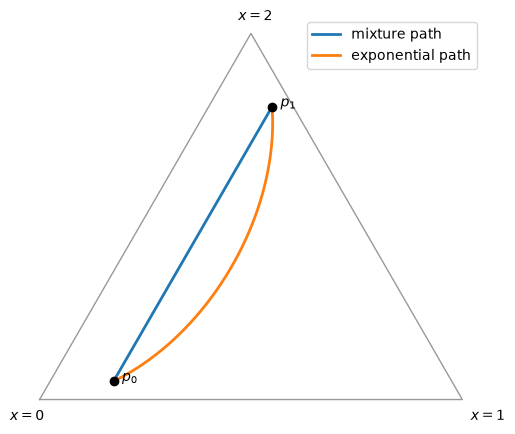
Fig. 23.1 Mixture and exponential paths#
We draw the simplex in probability coordinates, so the mixture path is straight.
The exponential path bends toward the middle outcome.
A geometric mean of two probabilities is small whenever either of them is small, which penalizes outcomes \(0\) and \(2\), each of which is improbable under one of the two distributions.
23.4. Two projections and two Pythagorean theorems#
23.4.1. The e-projection onto a linear family#
Let \(q\) be a distribution with full support, and let \(\mathcal{L} = \{ p : E_p[t(X)] = c \}\) be a linear family that contains a distribution with full support.
This holds exactly when \(c\) lies in the relative interior of the convex hull of the points \(t(x)\), that is, in its interior as a subset of the smallest affine subspace that contains it.
The same condition guarantees that the tilt in the theorem below exists.
Theorem 23.1 (e-projection)
The distribution \(p^* \in \mathcal{L}\) that minimizes \(D(p \| q)\) over \(p \in \mathcal{L}\) is the exponential tilt
with \(\theta\) chosen so that \(E_{p^*}[t(X)] = c\).
Moreover, for every \(p \in \mathcal{L}\),
Proof. Apply (23.1) with \((p, p^*, q)\) in place of \((p, q, r)\).
The cross term is
which proves (23.2).
Since \(D(p \| p^*) > 0\) unless \(p = p^*\), the tilt \(p^*\) is the unique minimizer.
When every member of \(\mathcal{L}\) puts zero probability on some outcomes, as for a die whose mean is \(6\), the e-projection still exists and is unique.
It lies outside the family of tilts, as a limit of tilts whose \(\theta\) diverges.
The e-projection of \(q\) lies on the exponential family generated by \(q\) and the statistic \(t\), at the point where that family crosses \(\mathcal{L}\).
In the proof, the cross term pairs a displacement \(p - p^*\) in probabilities, which lies along \(\mathcal{L}\), with a displacement \(\log p^* - \log q\) in log probabilities, which lies along the e-geodesic from \(q\) to \(p^*\).
This pairing is exactly the inner product defined by the Fisher information at \(p^*\).
For tangent vectors \(u\) and \(v\) at \(p^*\), expressed in probabilities, that inner product is \(\sum_x u(x) v(x) / p^*(x)\).
Take \(u = p - p^*\), the direction of \(\mathcal{L}\) toward \(p\), and take \(v\) to be the tangent at \(p^*\) of the e-geodesic \(p_s \propto q^{1 - s} (p^*)^s\).
Then \(v(x)/p^*(x) = \log p^*(x) - \log q(x) - D(p^* \| q)\), and the constant \(D(p^* \| q)\) drops out of the inner product because \(\sum_x u(x) = 0\).
The vanishing of the cross term is the precise sense in which the e-geodesic from \(q\) meets \(\mathcal{L}\) at a right angle.
We call \(p^*\) the e-projection because \(q\) reaches \(\mathcal{L}\) along an e-geodesic.
When \(q\) is the uniform distribution on \(m\) outcomes, \(D(p \| q) = \log m - H(p)\).
The e-projection of the uniform distribution is then the maximum entropy distribution of Exponential Family and Maximum Entropy, and (23.2) becomes the entropy-gap formula proved there.
For a general \(q\), the e-projection maximizes entropy relative to \(q\): it minimizes \(D(p \| q)\), the relative entropy of \(p\) with respect to \(q\).
23.4.2. The m-projection onto an exponential family#
Now let \(\mathcal{E} = \{ q_\theta \}\) be an exponential family with sufficient statistic \(t\) and base measure \(h\), and let \(p\) be any distribution that puts zero probability wherever \(h\) does.
Without that condition, \(D(p \| q_\theta)\) would be infinite for every \(\theta\).
Theorem 23.2 (m-projection)
If \(q_{\theta^*} \in \mathcal{E}\) matches the means of the sufficient statistic,
then \(q_{\theta^*}\) is the unique minimizer of \(D(p \| q_\theta)\) over \(\theta\), and, for every \(\theta\),
Proof. Apply (23.1) with \((p, q_{\theta^*}, q_\theta)\) in place of \((p, q, r)\).
Because \(\log q_{\theta^*}(x) - \log q_\theta(x) = (\theta^* - \theta) \cdot t(x) - F(\theta^*) + F(\theta)\), the cross term is
which proves (23.3).
Since \(D(q_{\theta^*} \| q_\theta) > 0\) unless \(\theta = \theta^*\), \(q_{\theta^*}\) is the unique minimizer.
Conversely, every minimizer matches moments.
Writing out the definitions gives \(D(p \| q_\theta) = F(\theta) - \theta \cdot E_p[t(X)]\) plus terms that do not depend on \(\theta\), so the first-order condition for a minimum is \(\nabla F(\theta) = E_p[t(X)]\).
An m-projection exists if and only if \(E_p[t(X)]\) lies in the range of \(\nabla F\).
For example, the m-projection onto the Bernoulli family of a distribution that puts all its probability on \(1\) does not exist.
For the same reason, a Bernoulli sample with no failures has no maximum likelihood estimate of the natural parameter.
The m-projection of \(p\) lies on the linear family of distributions that share \(p\)’s means of \(t\), at the point where that family crosses \(\mathcal{E}\).
Here the roles are reversed: the cross term pairs a displacement in probabilities along the m-geodesic from \(p\) to \(q_{\theta^*}\), which stays inside that linear family, with a displacement in natural parameters along \(\mathcal{E}\).
The m-geodesic from \(p\) meets \(\mathcal{E}\) at a right angle.
We call \(q_{\theta^*}\) the m-projection because \(p\) reaches \(\mathcal{E}\) along an m-geodesic.
In both theorems the projection is the vertex at the right angle, the point that appears in both terms on the right side.
Note
Conventions differ across the literature.
Check which argument of the KL divergence a source minimizes and which orthogonality condition it attaches to which Pythagorean identity.
Let \(p\), \(q\), and \(r\) be members of an exponential family with log-partition function \(F\) and Bregman divergence \(B_F\), as in Exponential Family and Maximum Entropy, with natural parameters \(\theta_p\), \(\theta_q\), \(\theta_r\) and expectation parameters \(\eta_p\), \(\eta_q\), \(\eta_r\).
Then
and
The two identities are the same statement with \(p\) and \(r\) interchanged: by (22.14) of Exponential Family and Maximum Entropy, the first says \(D(r \| p) = D(r \| q) + D(q \| p)\).
Writing the letters in the same order in the two notations attaches different orthogonality conditions.
Nielsen [2018] (in the text on pp. 322–323 and in the formula printed in Figure 2) and Nielsen [2020] (in the panel labels of Figure 6) pair each identity with the other’s condition; their definitions of e- and m-projections, and Theorem 6 of Nielsen [2020], are correct.
Let’s compute both projections for distributions on three outcomes with \(t(x) = x\).
For the e-projection, we take \(q = (0.6, 0.3, 0.1)\) and the linear family of distributions with mean \(1.2\).
For the m-projection, we take \(p = (0.5, 0.1, 0.4)\) and the exponential family generated by \(h = (0.2, 0.5, 0.3)\) and \(t\).
outcomes = np.arange(3.0)

# e-projection of q onto {p : E_p[X] = 1.2}
q_e = np.array([0.6, 0.3, 0.1])
θ_e, p_star = match_mean(q_e, outcomes, 1.2)

# members of the linear family: p_star plus multiples of (1, -2, 1),
# small enough to keep every probability positive
s_lo, s_hi = -min(p_star[0], p_star[2]), p_star[1] / 2
print("e-projection: D(p || q) and D(p || p*) + D(p* || q)")
for s in np.linspace(0.9 * s_lo, 0.9 * s_hi, 4):
    p = p_star + s * np.array([1.0, -2.0, 1.0])
    print(f"  {kl(p, q_e):.8f}   {kl(p, p_star) + kl(p_star, q_e):.8f}")

# m-projection of p onto the exponential family generated by h
h = np.array([0.2, 0.5, 0.3])
p_m = np.array([0.5, 0.1, 0.4])
θ_m, q_star = match_mean(h, outcomes, p_m @ outcomes)
print("\nm-projection: D(p || q_θ) and D(p || q*) + D(q* || q_θ)")
for θ in (-1.0, 0.0, 0.5, 2.0):
    q_θ = tilt(h, outcomes, θ)
    print(f"  {kl(p_m, q_θ):.8f}   {kl(p_m, q_star) + kl(q_star, q_θ):.8f}")
e-projection: D(p || q) and D(p || p*) + D(p* || q)
  0.80468819   0.80468819
  0.49622523   0.49622523
  0.46661670   0.46661670
  0.77420551   0.77420551

m-projection: D(p || q_θ) and D(p || q*) + D(q* || q_θ)
  0.45552607   0.45552607
  0.41227440   0.41227440
  0.57195583   0.57195583
  1.62161235   1.62161235
The figure shows the two projections.
In the left panel, the straight line is the linear family, and the curve through \(q\) is the exponential family generated by \(q\); the e-projection \(p^*\) is where they cross.
The thin curves are contours of \(D(p \| q)\) as a function of \(p\); the linear family is tangent to the contour through \(p^*\).
In the right panel, the curve is the exponential family generated by \(h\), and the straight line through \(p\) is the linear family of distributions that share \(p\)’s mean; the m-projection \(q^*\) is where they cross.
θ_grid = np.linspace(-6, 6, 400)


def family_curve(base, t, θ_grid):
    """Members of the exponential family generated by base and t."""
    return np.vstack([tilt(base, t, θ) for θ in θ_grid])


def linear_family(c, n=400):
    """Distributions on {0, 1, 2} with mean c."""
    lo, hi = max(0, c - 1), min(1, c / 2)   # range of p(2)
    p2 = np.linspace(lo, hi, n)
    p1 = c - 2 * p2
    return np.column_stack([1 - p1 - p2, p1, p2])


fig, axes = plt.subplots(1, 2, figsize=(11, 5))

ax = axes[0]
draw_simplex(ax)
# a barycentric grid of distributions with full support
k = 300
i, j = np.meshgrid(np.arange(1, k), np.arange(1, k))
inside = i + j < k
grid = np.column_stack([i[inside], j[inside], k - i[inside] - j[inside]]) / k
xy = to_triangle(grid)
ax.tricontour(xy[:, 0], xy[:, 1],
              np.sum(grid * np.log(grid / q_e), axis=1),
              levels=kl(p_star, q_e) * np.array([0.25, 0.5, 1.0, 1.5, 2.0]),
              colors="0.75", linewidths=0.8)
ax.plot(*to_triangle(linear_family(1.2)).T, lw=2,
        label=r"linear family $E[X] = 1.2$")
ax.plot(*to_triangle(family_curve(q_e, outcomes, θ_grid)).T, lw=2,
        label="exponential family through $q$")
for point, name in ((q_e, "$q$"), (p_star, "$p^*$")):
    ax.plot(*to_triangle(point)[0], "ko")
    ax.text(*to_triangle(point)[0] + [0.02, 0.01], name)
ax.set_title("e-projection", pad=18)
ax.legend(loc="upper left", fontsize=9, frameon=False)

ax = axes[1]
draw_simplex(ax)
ax.plot(*to_triangle(family_curve(h, outcomes, θ_grid)).T, lw=2, color="C1",
        label="exponential family through $h$")
ax.plot(*to_triangle(linear_family(p_m @ outcomes)).T, lw=2, color="C0",
        label=rf"linear family $E[X] = {p_m @ outcomes:.1f}$")
for point, name in ((p_m, "$p$"), (q_star, "$q^*$"), (h, "$h$")):
    ax.plot(*to_triangle(point)[0], "ko")
    ax.text(*to_triangle(point)[0] + [0.02, 0.01], name)
ax.set_title("m-projection", pad=18)
ax.legend(loc="upper left", fontsize=9, frameon=False)
plt.tight_layout()
plt.show()
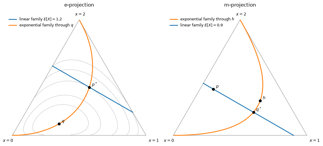
Fig. 23.2 The e-projection and the m-projection#
23.5. Maximum likelihood is an m-projection#
23.5.1. Correct specification#
Let \(x_1, \ldots, x_n\) be IID draws, and suppose that we fit an exponential family \(\{ q_\theta \}\) by maximum likelihood.
Exponential Family and Maximum Entropy shows that the maximum likelihood estimator \(\hat \theta\) matches the sample means of the sufficient statistic.
When the outcomes are discrete, let \(\hat p\) be the empirical distribution of the sample.
Then the average log likelihood is \(\sum_x \hat p(x) \log q_\theta(x) = -H(\hat p) - D(\hat p \| q_\theta)\).
Maximizing the likelihood is therefore minimizing \(D(\hat p \| q_\theta)\), because \(H(\hat p)\) does not depend on \(\theta\).
By Theorem 23.2, the maximum likelihood estimate is the m-projection of the empirical distribution onto the model.
Applying the Pythagorean theorem (23.3) with \(\hat p\) in the role of \(p\) gives \(D(\hat p \| q_\theta) - D(\hat p \| q_{\hat \theta}) = D(q_{\hat\theta} \| q_\theta)\), so that, for every \(\theta\),
where \(\ell_n\) is the log likelihood.
The identity (23.4) holds for continuous outcomes too: by the formulas of Exponential Family and Maximum Entropy, the left side equals \((\hat\theta - \theta) \cdot \bar t - F(\hat\theta) + F(\theta)\), and since \(\bar t = \nabla F(\hat \theta)\), this is the Bregman divergence \(B_F(\theta, \hat\theta) = D(q_{\hat\theta} \| q_\theta)\).
For an exponential family, whenever the maximum likelihood estimate exists, the likelihood-ratio statistic \(2[\ell_n(\hat\theta) - \ell_n(\theta_0)]\) equals \(2 n D(q_{\hat\theta} \| q_{\theta_0})\) exactly.
By Wilks’ theorem, when \(\theta_0\) is the true parameter this statistic is approximately \(\chi^2\) with as many degrees of freedom as there are parameters.
We check this with Poisson data, for which \(\hat \lambda = \bar x\) and \(D(q_{\hat\lambda} \| q_{\lambda_0}) = \hat\lambda \log(\hat\lambda/\lambda_0) - \hat\lambda + \lambda_0\).
λ0, n, R = 3.0, 50, 20_000
x = rng.poisson(λ0, size=(R, n))
λ_hat = x.mean(axis=1)

lr = 2 * (poisson.logpmf(x, λ_hat[:, None]).sum(axis=1)
          - poisson.logpmf(x, λ0).sum(axis=1))
two_n_kl = 2 * n * (λ_hat * np.log(λ_hat / λ0) - λ_hat + λ0)
print(f"max |LR - 2n KL| = {np.max(np.abs(lr - two_n_kl)):.2e}")
print(f"P(LR > 3.84) = {np.mean(lr > chi2.ppf(0.95, 1)):.4f}  (χ²_1: 0.05)")
max |LR - 2n KL| = 1.37e-13
P(LR > 3.84) = 0.0517  (χ²_1: 0.05)
The lecture Likelihood Ratio Processes compares two fixed models; by (23.4), within an exponential family, the KL divergence between the best-fitting model and any other model governs the likelihood ratio between them.
23.5.2. Misspecification#
Suppose now that the data come from a distribution \(p_0\) outside the model.
As Statistical Divergence Measures explains, under regularity conditions the maximum likelihood estimator then converges to the pseudo-true parameter \(\theta^*\) that minimizes \(D(p_0 \| q_\theta)\) [White, 1982].
Theorem 23.2 identifies it: for an exponential family, the pseudo-true parameter matches the population means of the sufficient statistic.
When we fit a normal distribution to data drawn from a mixture of normals, for example, the pseudo-true normal has the mean and variance of the mixture.
Let’s verify this, and the Pythagorean theorem (23.3), by numerical integration.
w, (μa, σa), (μb, σb) = 0.3, (-2.0, 0.7), (1.0, 1.0)


def log_mixture_pdf(x):
    return np.logaddexp(np.log(w) + norm.logpdf(x, μa, σa),
                        np.log(1 - w) + norm.logpdf(x, μb, σb))


def mixture_pdf(x):
    return np.exp(log_mixture_pdf(x))


def kl_mixture_normal(μ, σ):
    def integrand(x):
        log_p = log_mixture_pdf(x)
        return np.exp(log_p) * (log_p - norm.logpdf(x, μ, σ))
    return integrate.quad(integrand, -np.inf, np.inf, limit=200)[0]


def kl_normal(μ1, σ1, μ2, σ2):
    return np.log(σ2 / σ1) + (σ1**2 + (μ1 - μ2)**2) / (2 * σ2**2) - 0.5


μ_star = w * μa + (1 - w) * μb
σ_star = np.sqrt(w * (σa**2 + μa**2) + (1 - w) * (σb**2 + μb**2) - μ_star**2)
print(f"moment-matched normal: μ* = {μ_star:.4f}, σ* = {σ_star:.4f}")

print("\n   μ     σ    D(p0 || N)   D(p0 || N*) + D(N* || N)")
for μ, σ in ((0.0, 1.5), (μ_star, 1.0), (1.0, 2.0), (μ_star, σ_star)):
    lhs = kl_mixture_normal(μ, σ)
    rhs = kl_mixture_normal(μ_star, σ_star) + kl_normal(μ_star, σ_star, μ, σ)
    print(f"{μ:6.2f} {σ:5.2f} {lhs:12.6f} {rhs:16.6f}")
moment-matched normal: μ* = 0.1000, σ* = 1.6544

   μ     σ    D(p0 || N)   D(p0 || N*) + D(N* || N)
  0.00  1.50     0.108436         0.108436
  0.10  1.00     0.461027         0.461027
  1.00  2.00     0.229049         0.229049
  0.10  1.65     0.095958         0.095958
x_vals = np.linspace(-5, 5, 400)
fig, ax = plt.subplots()
ax.plot(x_vals, mixture_pdf(x_vals), lw=2, label="mixture $p_0$")
ax.plot(x_vals, norm.pdf(x_vals, μ_star, σ_star), lw=2, ls="--",
        label=rf"m-projection $N(\mu^*, \sigma^{{*2}})$")
ax.set_xlabel("$x$")
ax.legend()
plt.show()
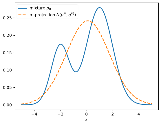
Fig. 23.3 Moment-matched normal for a bimodal mixture#
The moment-matched normal is the best normal approximation in the sense of \(D(p_0 \| q)\), even though it puts substantial probability between the two modes, where the mixture puts little.
The lecture Incorrect Models studies how a Bayesian learner who uses the wrong model behaves.
Gallant and Tauchen’s efficient method of moments builds an estimator on the fact that the expected score of the auxiliary model vanishes at the pseudo-true value.
23.6. Independence and mutual information#
Let \(p(x, y)\) be a joint distribution of two random variables that take finitely many values, with marginal distributions \(p_X\) and \(p_Y\).
The set of joint distributions under which \(X\) and \(Y\) are independent,
is an exponential family: its sufficient statistics are the indicators of the values of \(x\) and of \(y\) separately, and the means of these statistics are the two marginal distributions.
By Theorem 23.2, the m-projection of \(p\) onto \(\mathcal{E}_{\text{ind}}\) is the product of the marginals, \(p_X p_Y\).
The minimized divergence is the mutual information
the KL divergence of \(p\) from the nearest joint distribution under which \(X\) and \(Y\) are independent.
For any marginal distributions \(q_1\) and \(q_2\), the Pythagorean theorem (23.3) gives
and, because the logarithm of a product is a sum, the last term splits into \(D(p_X \| q_1) + D(p_Y \| q_2)\).
So
which splits the divergence of \(p\) from an independent model into a part due to dependence and parts due to the marginals.
p_xy = np.array([[0.20, 0.05, 0.05],
                 [0.05, 0.25, 0.05],
                 [0.02, 0.08, 0.25]])
p_x, p_y = p_xy.sum(axis=1), p_xy.sum(axis=0)
mutual_info = kl(p_xy, np.outer(p_x, p_y))
print(f"I(X; Y) = {mutual_info:.6f}")

for _ in range(3):
    q1, q2 = rng.dirichlet(np.ones(3), size=2)
    lhs = kl(p_xy, np.outer(q1, q2))
    rhs = mutual_info + kl(p_x, q1) + kl(p_y, q2)
    print(f"D(p || q1 q2) = {lhs:.6f},  decomposition = {rhs:.6f}")
I(X; Y) = 0.290227
D(p || q1 q2) = 0.956493,  decomposition = 0.956493
D(p || q1 q2) = 1.842041,  decomposition = 1.842041
D(p || q1 q2) = 1.551582,  decomposition = 1.551582
Mutual information is the measure of information flow in the theory of rational inattention initiated by Sims [2003].
Exercise 23.3 extends the decomposition to three random variables.
23.7. Maximum entropy and large deviations#
The maximum entropy distribution \(p^*\) of a die whose mean is \(4.5\) is the e-projection of the uniform distribution \(q\) onto the linear family \(\{ p : E_p[X] = 4.5 \}\).
We recompute it because we need it below.
faces = np.arange(1.0, 7.0)
q_die = np.full(6, 1 / 6)
θ_die, p_die = match_mean(q_die, faces, 4.5)
print("e-projection of the uniform distribution:", np.round(p_die, 4))
print(f"D(p* || q) = {kl(p_die, q_die):.4f}")
e-projection of the uniform distribution: [0.0544 0.0788 0.1142 0.1654 0.2398 0.3475]
D(p* || q) = 0.1782
Large deviations theory explains why the e-projection answers Jaynes’s question.
Sanov’s theorem concerns the empirical distribution \(\hat p_n\) of \(n\) IID draws from \(q\).
It says that, for a set \(\mathcal{S}\) of distributions that satisfies a mild regularity condition (for example, that \(\mathcal{S}\) is the closure of its interior),
where \(p_{\mathcal{S}}\) is the e-projection of \(q\) onto \(\mathcal{S}\).
The probability that the empirical distribution lands in \(\mathcal{S}\) decays exponentially, at the rate \(D(p_{\mathcal{S}} \| q)\).
When we roll a fair die \(n\) times, an average of at least \(4.5\) is the event that \(\hat p_n\) lies in the half-space \(\mathcal{S} = \{ p : E_p[X] \geq 4.5 \}\).
Because \(q\) has mean \(3.5\), the e-projection of \(q\) onto this half-space lies on its boundary, the linear family \(\{ p : E_p[X] = 4.5 \}\).
Along the straight line from any \(p\) with a larger mean toward \(q\), \(D(\cdot \| q)\) falls, because it is convex and zero at \(q\); the line passes through a point with mean \(4.5\).
The e-projection is therefore \(p^*\), and
The same calculation says how the rare event is most likely to happen: among all the ways that \(n\) fair rolls could produce an average of \(4.5\), overwhelmingly the most likely is that the frequencies of the faces resemble \(p^*\).
The conditional limit theorem makes this precise.
Suppose that we roll a fair die \(n\) times and learn only that the average number of spots was exactly \(4.5\), which requires \(n\) to be even.
Given this information, the distribution of the number of spots on the first roll converges to the e-projection \(p^*\) as \(n \to \infty\) [Csiszár, 1984, Van Campenhout and Cover, 1981].
Chapter 11 of Cover and Thomas [2006] proves both theorems.
We can check them exactly.
The distribution of the sum \(S_n\) of \(n\) rolls is an \(n\)-fold convolution, and
the formula on which Van Campenhout and Cover [1981] base their proof.
def sum_distribution(pmf, n):
    """Distribution of the sum of n IID draws from pmf on {1, ..., m}.

    Entry j of the result is the probability that the sum equals j + n.
    """
    dist = np.array([1.0])
    for _ in range(n):
        dist = np.convolve(dist, pmf)
    return dist


print("    n   P(X_1 = k | average = 4.5), k = 1, ..., 6     "
      "-log P(average ≥ 4.5)/n")
n_vals = [10, 20, 40, 80, 160, 320, 640]
rates = []
for n in n_vals:
    s = int(4.5 * n)
    dist_n1 = sum_distribution(q_die, n - 1)
    dist_n = np.convolve(dist_n1, q_die)
    cond = np.array([q_die[k - 1] * dist_n1[s - k - (n - 1)]
                     for k in range(1, 7)]) / dist_n[s - n]
    rates.append(-np.log(dist_n[s - n:].sum()) / n)
    print(f"{n:5d}   {np.round(cond, 4)}   {rates[-1]:.4f}")
print(f"  p* = {np.round(p_die, 4)}   D(p* || q) = {kl(p_die, q_die):.4f}")
    n   P(X_1 = k | average = 4.5), k = 1, ..., 6     -log P(average ≥ 4.5)/n
   10   [0.0473 0.077  0.1191 0.1755 0.2473 0.3338]   0.3244
   20   [0.0509 0.0779 0.1165 0.1704 0.2435 0.3408]   0.2656
   40   [0.0526 0.0784 0.1153 0.1679 0.2417 0.3441]   0.2296
   80   [0.0535 0.0786 0.1147 0.1666 0.2407 0.3458]   0.2079
  160   [0.0539 0.0787 0.1144 0.166  0.2402 0.3467]   0.1951
  320   [0.0541 0.0787 0.1143 0.1657 0.24   0.3471]   0.1877
  640   [0.0542 0.0787 0.1142 0.1656 0.2399 0.3473]   0.1835
  p* = [0.0544 0.0788 0.1142 0.1654 0.2398 0.3475]   D(p* || q) = 0.1782
fig, ax = plt.subplots()
ax.plot(n_vals, rates, "o-", label=r"$-\frac{1}{n}\log P(\bar X_n \geq 4.5)$")
ax.axhline(kl(p_die, q_die), color="k", ls="--", lw=1,
           label=r"$D(p^* \| q)$")
ax.set_xscale("log")
ax.set_xlabel("number of rolls $n$")
ax.legend()
plt.show()
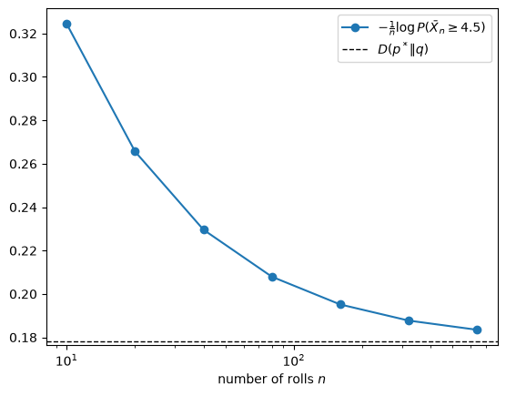
Fig. 23.4 Decay rate converges to \(D(p^* \| q)\)#
The conditional distributions converge quickly to \(p^*\); the decay rates converge more slowly, because the probabilities also contain factors that are polynomial in \(n\).
The large deviations results in Likelihood Ratio Processes and in the lecture on merging of opinions rest on the same mathematics.
23.8. Worst-case models in robust control#
Let \(\pi\) be a baseline probability distribution over states \(x\), and let \(u(x)\) be a decision maker’s utility.
A decision maker who fears that \(\pi\) is misspecified can evaluate prospects by the worst expected utility over alternative distributions \(q\), penalizing alternatives by their KL divergence from \(\pi\):
where \(\lambda > 0\) measures the decision maker’s confidence in \(\pi\).
These are the multiplier preferences of Hansen and Sargent [2001].
To solve (23.5), define the exponential tilt
Because \(\log q^*_\lambda(x) = \log \pi(x) - u(x)/\lambda - \log E_\pi \exp(-u(X)/\lambda)\), we have
or, for every \(q\),
so the worst-case distribution is \(q^*_\lambda\) and the value of (23.5) is \(-\lambda \log E_\pi \exp(-u(X)/\lambda)\).
Each worst-case model \(q^*_\lambda\) is also the e-projection of \(\pi\) onto the linear family \(\{ q : E_q[u(X)] = E_{q^*_\lambda}[u(X)] \}\): among all distributions that deliver that expected utility, it is closest to \(\pi\).
The value \(-\lambda \log E_\pi \exp(-u(X)/\lambda)\) is the risk-sensitive value function of Whittle [1990] and Hansen and Sargent [2008].
It is also an instance of the logit formula (22.12) of Exponential Family and Maximum Entropy, with \(v = -u\) and \(\tau = \lambda\).
The letters trade places: the baseline \(\pi\) here is the base distribution \(q\) there, and the distribution \(q\) chosen here is the vector \(\pi\) there.
Minimizing \(E_q[u] + \lambda D(q \| \pi)\) is maximizing \(E_q[-u] - \lambda D(q \| \pi)\), so the value of (23.5) is minus the left side of (22.12).
The worst-case models form a one-parameter exponential family that passes through \(\pi\), with sufficient statistic \(u\) and natural parameter \(-1/\lambda\).
As \(\lambda\) falls, the decision maker trusts \(\pi\) less, and the worst case moves along this family, putting more probability on states with low utility.
The example below has log utility over consumption, \(u(x) = \log x\), with the logarithm of consumption distributed \(N(0, 0.2^2)\) under \(\pi\).
Write \(z = \log x\); tilting the \(N(0, 0.2^2)\) density of \(z\) by \(\exp(-z/\lambda)\) gives the \(N(-0.2^2/\lambda, 0.2^2)\) density, so each worst case is again lognormal.
Then \(E_{q^*_\lambda}[u] = -0.2^2/\lambda\) and \(D(q^*_\lambda \| \pi) = 0.2^2/(2 \lambda^2)\).
We discretize log consumption on a grid wide enough to contain the worst cases we consider, and compare the results with these formulas.
σ_c = 0.2
log_c = np.linspace(-2.8, 0.8, 91)
π_base = norm.pdf(log_c, 0, σ_c)
π_base /= π_base.sum()
u_c = log_c                                # u(c) = log c


def worst_case(λ):
    return tilt(π_base, u_c, -1 / λ)


def multiplier_value(λ):
    return -λ * logsumexp(-u_c / λ, b=π_base)


λ_shown = (0.2, 0.05, 0.02)
print("    λ   E_q[u]  exact   D(q || π)   exact   E_q[u] + λ D   "
      "-λ log E exp(-u/λ)")
for λ in λ_shown:
    q = worst_case(λ)
    print(f"{λ:5.2f} {q @ u_c:8.4f} {-σ_c**2 / λ:6.2f} {kl(q, π_base):10.4f} "
          f"{σ_c**2 / (2 * λ**2):7.2f} {q @ u_c + λ * kl(q, π_base):12.4f} "
          f"{multiplier_value(λ):16.4f}")
    λ   E_q[u]  exact   D(q || π)   exact   E_q[u] + λ D   -λ log E exp(-u/λ)
 0.20  -0.2000  -0.20     0.5000    0.50      -0.1000          -0.1000
 0.05  -0.8000  -0.80     8.0000    8.00      -0.4000          -0.4000
 0.02  -2.0000  -2.00    49.9991   50.00      -1.0000          -1.0000
fig, axes = plt.subplots(1, 2, figsize=(11, 4))
ax = axes[0]
ax.plot(log_c, π_base, "k", lw=2, label=r"baseline $\pi$")
for λ in λ_shown:
    ax.plot(log_c, worst_case(λ), label=rf"worst case, $\lambda$ = {λ}")
ax.set_xlabel("log consumption")
ax.set_ylabel("probability")
ax.legend()

ax = axes[1]
λ_vals = np.geomspace(0.02, 2, 100)
rel_entropies = [kl(worst_case(λ), π_base) for λ in λ_vals]
utilities = [worst_case(λ) @ u_c for λ in λ_vals]
ax.plot(rel_entropies, utilities, lw=3, alpha=0.5, label="on the grid")
D_vals = np.linspace(0, max(rel_entropies), 200)
ax.plot(D_vals, -σ_c * np.sqrt(2 * D_vals), "k--", lw=1,
        label=r"exact, $-0.2\sqrt{2D}$")
ax.set_xlabel(r"$D(q^*_\lambda \| \pi)$")
ax.set_ylabel(r"$E_{q^*_\lambda}[u(X)]$")
ax.set_title("worst-case expected utility and relative entropy")
ax.legend()
plt.tight_layout()
plt.show()
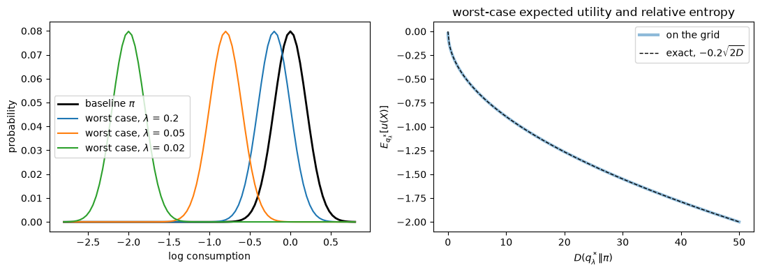
Fig. 23.5 Worst-case distributions under multiplier preferences#
The right panel traces the worst-case expected utility against the relative entropy of the worst case; eliminating \(\lambda\) from the two formulas above gives \(E_{q^*_\lambda}[u] = -0.2 \sqrt{2 D(q^*_\lambda \| \pi)}\).
Each point on this curve also solves the problem of minimizing expected utility subject to the constraint \(D(q \| \pi) \leq \kappa\), with \(\kappa\) equal to the point’s horizontal coordinate; Exercise 23.2 asks you to verify this.
These are the constraint preferences studied in the lecture Risk and Model Uncertainty, which writes \(\theta\) for our \(\lambda\) and \(\eta\) for our \(\kappa\).
Another advanced lecture uses such worst-case models to ask whether asset prices reflect risk aversion or mistaken beliefs.
Exponential tilting also appears in Mean of a Likelihood Ratio Process, where it delivers efficient importance samplers.
23.9. Matrix balancing: RAS and Sinkhorn#
23.9.1. Updating an input–output table#
Input–output analysts often need to update a table.
Input-Output Models describes such tables.
A table \(Q\) of flows of goods among industries is available for a base year.
For a later year, the analyst knows only the row totals \(r\) (each industry’s sales to other industries) and the column totals \(c\) (each industry’s purchases from other industries).
In this section, \(r\) and \(c\) denote vectors of totals.
Matrix balancing finds a table that has given totals and stays close to a base table.
A natural estimate of the new table is the matrix \(P^*\) that has these totals and minimizes \(D(P \| Q)\).
Because \(P\) and \(Q\) need not have the same total, we use the generalized KL divergence for nonnegative arrays,
which is nonnegative and zero only when \(P = Q\), and for which the three-point identity (23.1) still holds.
The set of matrices with row totals \(r\) is a linear family, and so is the set of matrices with column totals \(c\).
The matrix \(P^*\) is the e-projection of \(Q\) onto their intersection.
The argument that proved Theorem 23.1, with the indicators of the rows and of the columns as the statistics \(t\), applies here.
It shows that if a matrix of the biproportional form
with positive vectors \(a\) and \(b\), has the required totals, then it is \(P^*\), because the cross term in (23.1) becomes \(\sum_i \log a_i \, (r_i - r_i) + \sum_j \log b_j \, (c_j - c_j) = 0\).
Such a matrix exists when every entry of \(Q\) is positive, \(r\) and \(c\) are positive, and \(\sum_i r_i = \sum_j c_j\) [Bacharach, 1970].
The RAS method finds \(a\) and \(b\) by alternately rescaling the rows of the current table to match \(r\) and its columns to match \(c\); each rescaling is the e-projection of the current table onto one of the two linear families.
Deming and Stephan [1940] proposed this algorithm, which statisticians call iterative proportional fitting, for adjusting census tables to known marginal totals.
Stone and Brown [1962] used it to update input–output tables.
Ireland and Kullback [1968] identified its limit as the table that minimizes the KL divergence from the base table, but their proof of convergence was incomplete.
Bacharach [1970] studied its properties for input–output analysis.
Csiszár [1975] gave a complete proof that it converges.
The Pythagorean theorem explains why the algorithm converges.
Let \(P\) be any matrix with both sets of totals that is zero wherever \(Q\) is zero, so that \(D(P \| Q) < \infty\).
Because each rescaling is an e-projection onto a linear family that contains \(P\), (23.2) gives
where \(P^{(k)}\) is the table after \(k\) rescalings, counting a row rescaling and a column rescaling as two steps.
In particular, the divergence of \(P^*\) from the iterates falls at every step.
Summing gives \(D(P \| Q) = D(P \| P^{(k)}) + \sum_{j < k} D(P^{(j + 1)} \| P^{(j)})\), where the sum does not depend on \(P\).
Taking \(P = P^*\) shows that \(\sum_k D(P^{(k + 1)} \| P^{(k)}) \leq D(P^* \| Q)\), so successive iterates become arbitrarily close, and every limit point \(\bar P\) of the iterates has both sets of totals.
Letting \(k \to \infty\) along a subsequence that converges to \(\bar P\), with \(P = \bar P\), gives \(D(\bar P \| Q) = \sum_k D(P^{(k + 1)} \| P^{(k)})\), which by the same identity is at most \(D(P \| Q)\) for every admissible \(P\).
So every limit point is the minimizer \(P^*\), and the iterates converge to it [Csiszár, 1975].
The argument does not need the biproportional form; when \(Q\) has zeros, a biproportional solution may not exist.
For example, let \(Q\) have rows \((1, 1)\) and \((0, 1)\), and let all totals equal \(1\).
The only admissible table is the identity matrix.
It is not of the form \(a_i Q_{ij} b_j\) with positive \(a\) and \(b\), but RAS still converges to it.
def gen_kl(P, Q):
    """Generalized KL divergence of nonnegative arrays."""
    mask = P > 0
    return np.sum(P[mask] * np.log(P[mask] / Q[mask])) - P.sum() + Q.sum()


def ras(Q, r, c, tol=1e-12, max_iter=10_000):
    """Rescale rows and columns of Q to match totals r and c."""
    if not np.isclose(r.sum(), c.sum()):
        raise ValueError("row and column totals must have the same sum")
    P = Q.copy()
    history = [P.copy()]
    for _ in range(max_iter):
        P = P * (r / P.sum(axis=1))[:, None]
        history.append(P.copy())
        P = P * (c / P.sum(axis=0))[None, :]
        history.append(P.copy())
        if np.max(np.abs(P.sum(axis=1) - r)) < tol * r.sum():
            break
    else:
        warnings.warn("RAS did not converge")
    return P, history


Q_io = np.array([[20.0, 10.0, 5.0],
                 [8.0, 30.0, 12.0],
                 [6.0, 9.0, 25.0]])
r_new = np.array([40.0, 55.0, 45.0])
c_new = np.array([38.0, 52.0, 50.0])

P_io, history = ras(Q_io, r_new, c_new)
print("base table:\n", Q_io)
print("updated table:\n", np.round(P_io, 3))
print("row totals:", np.round(P_io.sum(axis=1), 6),
      " column totals:", np.round(P_io.sum(axis=0), 6))
base table:
 [[20. 10.  5.]
 [ 8. 30. 12.]
 [ 6.  9. 25.]]
updated table:
 [[22.787 10.972  6.241]
 [ 8.793 31.755 14.452]
 [ 6.42   9.273 29.307]]
row totals: [40. 55. 45.]  column totals: [38. 52. 50.]
The ratio \(P^*_{ij} / Q_{ij} = a_i b_j\) factors into a row effect times a column effect.
The name RAS describes this: the updated table is \(R A S\), with \(A\) the base table and \(R\) and \(S\) diagonal matrices of row and column multipliers, our \(a\) and \(b\).
If the ratio \(R_{ij} = P^*_{ij}/Q_{ij}\) factors as \(a_i b_j\), then \(R_{ij} = R_{i1} R_{1j} / R_{11}\), so dividing \(R_{ij}\) by \(R_{i1} R_{1j} / R_{11}\) leaves a matrix of ones.
ratio = P_io / Q_io
print("P*/Q divided by its first column and first row:")
print(np.round(ratio / np.outer(ratio[:, 0], ratio[0, :] / ratio[0, 0]), 10))
P*/Q divided by its first column and first row:
[[1. 1. 1.]
 [1. 1. 1.]
 [1. 1. 1.]]
The divergence of \(P^*\) from the iterates falls monotonically until it reaches the level of rounding error; the figure omits values below that level.
divergences = np.array([gen_kl(P_io, P) for P in history])
steps = np.arange(len(divergences))
keep = divergences > 1e-12
fig, ax = plt.subplots()
ax.semilogy(steps[keep], divergences[keep], "o-")
ax.set_xlabel("rescaling step $k$")
ax.set_ylabel(r"$D(P^* \| P^{(k)})$")
plt.show()
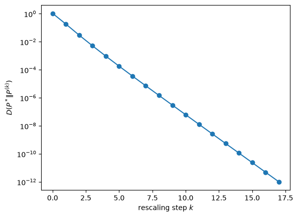
Fig. 23.6 Convergence of the RAS algorithm#
We check the Pythagorean theorem (23.2) for other tables with the same totals.
# add multiples of a pattern with zero row and column sums
pattern = np.array([[1.0, -1.0, 0.0], [-1.0, 1.0, 0.0], [0.0, 0.0, 0.0]])
for s in (-3.0, 2.0, 5.0):
    P_other = P_io + s * pattern
    print(f"D(P || Q) = {gen_kl(P_other, Q_io):.6f},  "
          f"D(P || P*) + D(P* || Q) = "
          f"{gen_kl(P_other, P_io) + gen_kl(P_io, Q_io):.6f}")
D(P || Q) = 2.259577,  D(P || P*) + D(P* || Q) = 2.259577
D(P || Q) = 1.655902,  D(P || P*) + D(P* || Q) = 1.655902
D(P || Q) = 5.132448,  D(P || P*) + D(P* || Q) = 5.132448
23.9.2. Entropy-regularized optimal transport#
Optimal Transport studies the problem of choosing a transport plan \(P\) with row totals \(p\) and column totals \(q\) (the notation of that lecture) to minimize the total cost \(\sum_{i, j} C_{ij} P_{ij}\).
Adding \(\varepsilon\) times the negative entropy of the plan gives the entropy-regularized problem
With \(K_{ij} = \exp(-C_{ij}/\varepsilon)\), the objective equals \(\varepsilon \, D(P \| K) - \varepsilon \sum_{ij} K_{ij}\).
The regularized problem therefore finds the e-projection of the matrix \(K\) onto the set of plans with the required totals.
The plan has the biproportional form \(P_{ij} = a_i K_{ij} b_j = a_i \exp(-C_{ij}/\varepsilon) b_j\), the same exponential tilting that solves (22.12) in Exponential Family and Maximum Entropy.
The rescaling algorithm of RAS solves it; in this setting the algorithm goes by the name Sinkhorn’s algorithm [Sinkhorn, 1964].
Cuturi [2013] showed that Sinkhorn’s algorithm makes large optimal transport problems tractable.
Galichon [2016] and Galichon and Salanié [2022] explain how the matching model of Choo and Siow [2006], in which agents have logit preferences over partners, leads to problems of this form.
When every agent is matched, the Choo–Siow model is exactly an entropy-regularized transport problem with fixed totals.
When \(\varepsilon\) is small, the entries of \(K\) are tiny, so we carry out the rescalings in logarithms.
We use the example of Optimal Transport, solve the linear program with linprog, and compare its solution with the solutions of the regularized problem for decreasing \(\varepsilon\).
def sinkhorn(C, p, q, ε, tol=1e-10, max_iter=100_000):
    """Entropy-regularized optimal transport by rescaling in logs."""
    log_K = -C / ε
    log_a, log_b = np.zeros(len(p)), np.zeros(len(q))
    for _ in range(max_iter):
        log_a = np.log(p) - logsumexp(log_K + log_b[None, :], axis=1)
        log_b = np.log(q) - logsumexp(log_K + log_a[:, None], axis=0)
        P = np.exp(log_a[:, None] + log_K + log_b[None, :])
        if np.max(np.abs(P.sum(axis=1) - p)) < tol * p.sum():
            break
    else:
        warnings.warn("Sinkhorn's algorithm did not converge")
    return P


p_ot = np.array([50.0, 100.0, 150.0])
q_ot = np.array([25.0, 115.0, 60.0, 30.0, 70.0])
C_ot = np.array([[10.0, 15.0, 20.0, 20.0, 40.0],
                 [20.0, 40.0, 15.0, 30.0, 30.0],
                 [30.0, 35.0, 40.0, 55.0, 25.0]])
m, n = C_ot.shape

# the linear program of the optimal transport lecture
A_eq = np.vstack([np.kron(np.ones((1, n)), np.identity(m)),
                  np.kron(np.identity(n), np.ones((1, m)))])
res_lp = linprog(C_ot.reshape(-1, order="F"), A_eq=A_eq[:-1],
                 b_eq=np.hstack([p_ot, q_ot])[:-1])
P_lp = res_lp.x.reshape((m, n), order="F")

print(f"linear program: cost = {res_lp.fun:.3f}")
for ε in (10.0, 3.0, 1.0, 0.1):
    P_ε = sinkhorn(C_ot, p_ot, q_ot, ε)
    print(f"ε = {ε:5.1f}: cost = {np.sum(C_ot * P_ε):9.3f}")
linear program: cost = 7225.000
ε =  10.0: cost =  7947.977
ε =   3.0: cost =  7261.065
ε =   1.0: cost =  7225.002
ε =   0.1: cost =  7225.000
As \(\varepsilon \to 0\), the cost of the regularized solution converges to the minimal cost.
The regularized plans need not converge to the plan that linprog reports.
P_small = sinkhorn(C_ot, p_ot, q_ot, 0.05)
print("linprog plan:\n", np.round(P_lp, 2))
print("limit of regularized plans:\n", np.round(P_small, 2))


def plan_entropy(P):
    """Entropy of the plan, normalized to be a probability distribution."""
    P = P[P > 1e-12] / P.sum()
    return -np.sum(P * np.log(P))


print(f"costs: {np.sum(C_ot * P_lp):.3f} and {np.sum(C_ot * P_small):.3f}")
print(f"entropies: {plan_entropy(P_lp):.4f} and {plan_entropy(P_small):.4f}")
linprog plan:
 [[ 0. 50.  0.  0.  0.]
 [10.  0. 60. 30.  0.]
 [15. 65.  0.  0. 70.]]
limit of regularized plans:
 [[ 3.42 41.14  0.    5.44  0.  ]
 [15.44  0.   60.   24.56  0.  ]
 [ 6.14 73.86  0.    0.   70.  ]]
costs: 7225.000 and 7225.000
entropies: 1.7849 and 1.8399
This problem has many optimal plans.
linprog typically returns a vertex of the set of optimal plans.
The regularized plans converge to the optimal plan with the largest entropy [Cominetti and San Martín, 1994].
That limit is itself an e-projection.
By complementary slackness, the optimal plans are exactly the plans with the required totals that use only the cells that some optimal plan uses.
The optimal plan with the largest entropy is the result of applying the RAS method to the matrix that has ones in those cells and zeros elsewhere.
support = (P_small > 1e-6 * p_ot.sum()).astype(float)
P_maxent, _ = ras(support, p_ot, q_ot)
print("RAS applied to the optimal support:\n", np.round(P_maxent, 2))
print(f"cost = {np.sum(C_ot * P_maxent):.3f}, "
      f"entropy = {plan_entropy(P_maxent):.4f}")
RAS applied to the optimal support:
 [[ 3.42 41.14  0.    5.44  0.  ]
 [15.44  0.   60.   24.56  0.  ]
 [ 6.14 73.86  0.    0.   70.  ]]
cost = 7225.000, entropy = 1.8399
23.10. Chernoff information#
Statistical Divergence Measures defines the Chernoff entropy, which information theorists call the Chernoff information, of densities \(f\) and \(g\) as
and Likelihood Ratio Processes shows that it governs the rate at which the probability of a mistaken model selection falls as observations accumulate.
We assume that \(f\) and \(g\) are distinct and have the same support, so that \(\log \rho\), which is zero at \(\phi = 0\) and \(\phi = 1\) and strictly convex, attains its minimum at an interior point \(\phi^*\).
Information projections give the Chernoff information a geometric interpretation [Nielsen, 2013].
The normalized geometric mixtures
form the exponential path between \(g\) (at \(\phi = 0\)) and \(f\) (at \(\phi = 1\)).
This path is a one-parameter exponential family with sufficient statistic \(\log(f/g)\), natural parameter \(\phi\), and log-partition function \(\log \rho(\phi)\).
At the minimizer \(\phi^*\) of \(\log \rho\), the derivative of the log-partition function vanishes, so \(E_{p_{\phi^*}}[\log(f(X)/g(X))] = 0\).
Since \(D(p_\phi \| f) = (\phi - 1) E_{p_\phi}[\log(f/g)] - \log \rho(\phi)\) and \(D(p_\phi \| g) = \phi E_{p_\phi}[\log(f/g)] - \log \rho(\phi)\), it follows that
The Chernoff information is the common value of \(D(p_{\phi^*} \| f)\) and \(D(p_{\phi^*} \| g)\), where \(p_{\phi^*}\) is the unique point on the exponential path between \(f\) and \(g\) that is equally far from both.
Because \(D(p \| f) - D(p \| g) = -E_p[\log(f(X)/g(X))]\), a distribution is equally far from \(f\) and \(g\) exactly when the log-likelihood ratio has mean zero under it.
The linear family \(\mathcal{L}_0 = \{ p : E_p[\log(f/g)] = 0 \}\) is the analog of a perpendicular bisector.
The point \(p_{\phi^*}\) is the e-projection of both \(f\) and \(g\) onto \(\mathcal{L}_0\): the e-projection of \(f\) is a tilt of \(f\) by \(\exp(\theta \log(f/g))\), which lies on the exponential path, and \(p_{\phi^*}\) is the only point of the path in \(\mathcal{L}_0\).
This explains why Chernoff information governs error rates.
A test that selects the model with the higher likelihood errs when the sample average of \(\log(f/g)\) has the wrong sign.
If the data come from \(f\), that is the event that the empirical distribution lies in the half-space \(\{ p : E_p[\log(f/g)] \leq 0 \}\).
Since \(E_f[\log(f/g)] = D(f \| g) > 0\), the e-projection of \(f\) onto the half-space lies on its boundary \(\mathcal{L}_0\), as in the dice example, and the probability of the event decays at rate \(D(p_{\phi^*} \| f) = C(f, g)\).
For distributions on a finite set this is Sanov’s theorem; for densities, Cramér’s theorem applied to the sample mean of \(\log(f(X)/g(X))\) gives the same rate, because its rate function at zero is \(-\min_\phi \log \rho(\phi)\).
If the data come from \(g\), the error event is \(\{ p : E_p[\log(f/g)] \geq 0 \}\), and the rate is \(D(p_{\phi^*} \| g) = C(f, g)\).
We use the two Beta distributions of Statistical Divergence Measures, \(f = \) Beta(1, 1) and \(g = \) Beta(3, 1.2).
Because the Beta family is an exponential family, the exponential path between two Beta distributions stays in the Beta family: \(p_\phi\) is the Beta distribution whose parameters are \(\phi\) times those of \(f\) plus \(1 - \phi\) times those of \(g\).
All the quantities we need have closed forms.
fa, fb, ga, gb = 1.0, 1.0, 3.0, 1.2


def path_params(ϕ):
    return ϕ * fa + (1 - ϕ) * ga, ϕ * fb + (1 - ϕ) * gb


def log_ρ(ϕ):
    return (betaln(*path_params(ϕ)) - ϕ * betaln(fa, fb)
            - (1 - ϕ) * betaln(ga, gb))


def kl_beta(a1, b1, a2, b2):
    """KL divergence of Beta(a1, b1) from Beta(a2, b2)."""
    return (betaln(a2, b2) - betaln(a1, b1) + (a1 - a2) * digamma(a1)
            + (b1 - b2) * digamma(b1) + (a2 - a1 + b2 - b1) * digamma(a1 + b1))


res_ϕ = minimize_scalar(log_ρ, bounds=(1e-8, 1 - 1e-8), method="bounded",
                        options={"xatol": 1e-12})
ϕ_star, C_fg = res_ϕ.x, -res_ϕ.fun
print(f"ϕ* = {ϕ_star:.6f},  Chernoff information C(f, g) = {C_fg:.6f}")
print(f"D(p_ϕ* || f) = {kl_beta(*path_params(ϕ_star), fa, fb):.6f}")
print(f"D(p_ϕ* || g) = {kl_beta(*path_params(ϕ_star), ga, gb):.6f}")
print("p_ϕ* = Beta({:.4f}, {:.4f})".format(*path_params(ϕ_star)))
ϕ* = 0.596854,  Chernoff information C(f, g) = 0.121186
D(p_ϕ* || f) = 0.121186
D(p_ϕ* || g) = 0.121186
p_ϕ* = Beta(1.8063, 1.0806)
The Chernoff information agrees with the value computed by numerical integration in Statistical Divergence Measures.
ϕ_vals = np.linspace(0.001, 0.999, 300)
fig, axes = plt.subplots(1, 2, figsize=(11, 4))

ax = axes[0]
ax.plot(ϕ_vals, [kl_beta(*path_params(ϕ), fa, fb) for ϕ in ϕ_vals],
        label=r"$D(p_\phi \| f)$")
ax.plot(ϕ_vals, [kl_beta(*path_params(ϕ), ga, gb) for ϕ in ϕ_vals],
        label=r"$D(p_\phi \| g)$")
ax.plot(ϕ_vals, -log_ρ(ϕ_vals), "k--", lw=1, label=r"$-\log\rho(\phi)$")
ax.plot([ϕ_star], [C_fg], "ko")
ax.axvline(ϕ_star, color="0.7", lw=0.8)
ax.set_xlabel(r"$\phi$")
ax.set_ylim(0, 0.6)
ax.legend()

ax = axes[1]
z = np.linspace(0.001, 0.999, 300)
for (a_, b_), label in (((fa, fb), "$f$"), ((ga, gb), "$g$"),
                        (path_params(ϕ_star), r"$p_{\phi^*}$")):
    ax.plot(z, np.exp((a_ - 1) * np.log(z) + (b_ - 1) * np.log(1 - z)
                      - betaln(a_, b_)), lw=2, label=label)
ax.set_xlabel("$x$")
ax.legend()
plt.tight_layout()
plt.show()
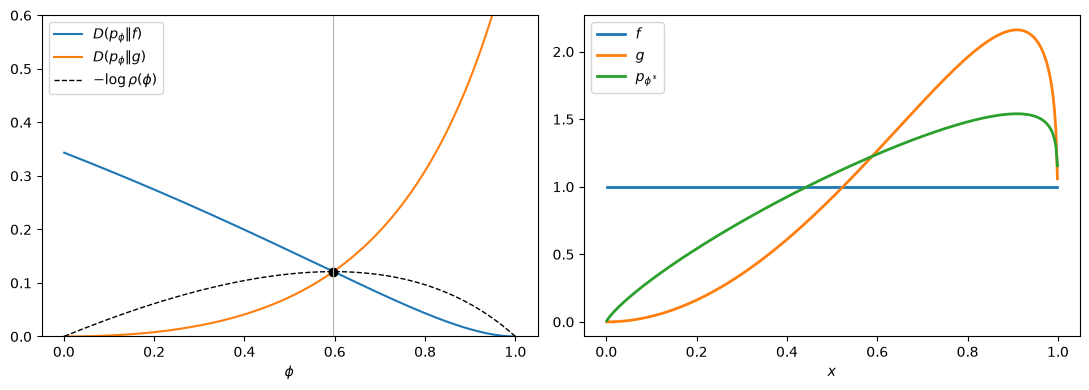
Fig. 23.7 Point equally far from both distributions#
In the left panel, the two divergences cross at \(\phi^*\), where their common value equals the maximum of \(-\log \rho(\phi)\), the Chernoff information.
In the right panel, \(p_{\phi^*}\) lies between \(f\) and \(g\).
23.11. Concluding remarks#
KL divergence is not a distance.
It has a geometry with two kinds of straight lines, mixtures and normalized geometric mixtures, and two corresponding kinds of projection.
The e-projection onto a set defined by moment conditions is an exponential tilt, and the m-projection onto an exponential family matches moments; each is unique and satisfies a Pythagorean theorem.
The lecture applied m-projections to maximum likelihood estimation and mutual information, and e-projections to maximum entropy and large deviations, robust control, the updating of input–output tables, optimal transport, and Chernoff information.
The worst-case models of robust control, the biproportional tables of RAS, and the regularized transport plans are all exponential tilts of the kind that attains the logit formula (22.12) of Exponential Family and Maximum Entropy.
Other applications include the EM algorithm, which Csiszár and Tusnády [1984] interpret as alternating projections, and the hierarchical decomposition of interactions among many random variables of Amari [2001], which Exercise 23.3 takes up.
23.12. Exercises#
Exercise 23.1
Survey statisticians and econometricians often reweight a sample so that it matches a population moment known from another source.
Let \(x_1, \ldots, x_n\) be a sample whose average differs from a known population mean \(\mu\).
Two ways to choose weights \(w_1, \ldots, w_n\) that sum to one and satisfy \(\sum_i w_i x_i = \mu\) are
exponential tilting: choose \(w\) to minimize \(D(w \| q)\), where \(q\) puts weight \(1/n\) on each observation; and
empirical likelihood: choose \(w\) to minimize \(D(q \| w)\), equivalently to maximize \(\sum_i \log w_i\).
Show that exponential tilting is an e-projection and that its weights have the form \(w_i \propto \exp(\theta x_i)\).
Show that the empirical likelihood weights have the form \(w_i = 1 / \left( n (1 + \gamma (x_i - \mu)) \right)\) for a scalar \(\gamma\).
Draw a sample of \(n = 200\) pairs \((x_i, y_i)\) with \(x_i\) lognormal and \(y_i = 1 + 0.5 x_i + e_i\), where \(e_i\) is normal noise. Compute both sets of weights so that the weighted mean of \(x\) equals \(1.2\) times its sample mean, compare the weights, and compare the two reweighted estimates of the mean of \(y\).
Kitamura and Stutzer [1997] and Owen [1988] develop estimators based on these two kinds of weights.
Solution
Here is one solution.
For part 1, the set of weight vectors with \(\sum_i w_i x_i = \mu\) is a linear family, so minimizing \(D(w \| q)\) over it is an e-projection; by Theorem 23.1, \(w_i \propto q_i \exp(\theta x_i) \propto \exp(\theta x_i)\).
Minimizing \(D(q \| w)\) is instead an m-projection of \(q\) onto the linear family; our theorems do not cover it.
For part 2, the Lagrangian of maximizing \(\sum_i \log w_i\) subject to \(\sum_i w_i = 1\) and \(\sum_i w_i (x_i - \mu) = 0\) has first-order conditions \(1/w_i = \alpha + \beta (x_i - \mu)\).
Multiplying by \(w_i\) and summing gives \(n = \alpha\), so \(w_i = 1/(n(1 + \gamma (x_i - \mu)))\) with \(\gamma = \beta / n\).
For part 3, we solve for \(\theta\) and \(\gamma\) by root finding.
rng_w = np.random.default_rng(11)
n = 200
x = rng_w.lognormal(0.0, 0.5, size=n)
y = 1 + 0.5 * x + rng_w.normal(0, 0.3, size=n)
μ = 1.2 * x.mean()
q_n = np.full(n, 1 / n)

θ_et, w_et = match_mean(q_n, x, μ, bracket=(-20, 20))

# γ must keep every weight positive
lo, hi = -1 / (x.max() - μ), -1 / (x.min() - μ)
γ_el = brentq(lambda γ: np.sum((x - μ) / (1 + γ * (x - μ))),
              lo + 1e-9, hi - 1e-9)
w_el = 1 / (n * (1 + γ_el * (x - μ)))

for name, wts in (("exponential tilting", w_et),
                  ("empirical likelihood", w_el)):
    print(f"{name:21}: sum {wts.sum():.6f}, weighted mean of x {wts @ x:.4f} "
          f"(target {μ:.4f}), weighted mean of y {wts @ y:.4f}")
print(f"unweighted mean of y: {y.mean():.4f}")

order = np.argsort(x)
fig, ax = plt.subplots()
ax.plot(x[order], n * w_et[order], "o-", ms=3, label="exponential tilting")
ax.plot(x[order], n * w_el[order], "s--", ms=3, label="empirical likelihood")
ax.set_xlabel("$x_i$")
ax.set_ylabel(r"$n \times$ weight")
ax.legend()
plt.show()
exponential tilting  : sum 1.000000, weighted mean of x 1.3456 (target 1.3456), weighted mean of y 1.7088
empirical likelihood : sum 1.000000, weighted mean of x 1.3456 (target 1.3456), weighted mean of y 1.6977
unweighted mean of y: 1.5826
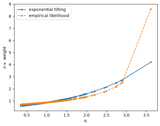
Both sets of weights raise the weighted mean of \(y\) by roughly half the change in the mean of \(x\).
Given the \(x_i\), the linear relationship \(y = 1 + 0.5 x + e\) makes the expected change exactly half; departures come from the noise \(e_i\).
The two estimates differ because the weights differ.
Exponential tilting weights rise exponentially with \(x\), while empirical likelihood weights rise more gently at first and then much more steeply for the largest observations.
Exercise 23.2
Consider the constraint version of the robust decision problem of the lecture:
Use the identity \(E_q[u] + \lambda D(q \| \pi) = \lambda D(q \| q^*_\lambda) - \lambda \log E_\pi \exp(-u/\lambda)\) to show that if \(\lambda > 0\) satisfies \(D(q^*_\lambda \| \pi) = \kappa\), then \(q^*_\lambda\) solves the constraint problem.
For the consumption example of the lecture and \(\kappa \in \{0.01, 0.05, 0.2\}\), find \(\lambda\) and the minimized expected utility.
For \(\kappa = 0.05\), check your answer by minimizing expected utility over all distributions on the consumption grid subject to \(D(q \| \pi) \leq \kappa\) with a general-purpose constrained optimizer.
Solution
Here is one solution.
For part 1, let \(q\) satisfy \(D(q \| \pi) \leq \kappa = D(q^*_\lambda \| \pi)\).
The identity gives
where the last equality applies the identity at \(q = q^*_\lambda\).
So no feasible \(q\) does better than \(q^*_\lambda\).
For part 2, \(D(q^*_\lambda \| \pi)\) falls as \(\lambda\) rises, so we can find \(\lambda\) by root finding on \(\log \lambda\).
def λ_for_entropy(κ):
    log_λ = brentq(lambda s: kl(worst_case(np.exp(s)), π_base) - κ, -6, 3)
    return np.exp(log_λ)


for κ in (0.01, 0.05, 0.2):
    λ = λ_for_entropy(κ)
    print(f"κ = {κ:4.2f}: λ = {λ:.4f} (exact {σ_c / np.sqrt(2 * κ):.4f}), "
          f"min E_q[u] = {worst_case(λ) @ u_c:.5f} "
          f"(exact {-σ_c * np.sqrt(2 * κ):.5f})")
κ = 0.01: λ = 1.4140 (exact 1.4142), min E_q[u] = -0.02830 (exact -0.02828)
κ = 0.05: λ = 0.6324 (exact 0.6325), min E_q[u] = -0.06326 (exact -0.06325)
κ = 0.20: λ = 0.3162 (exact 0.3162), min E_q[u] = -0.12650 (exact -0.12649)
The exact values come from the formulas for the lognormal example: \(D(q^*_\lambda \| \pi) = 0.2^2/(2\lambda^2) = \kappa\) gives \(\lambda = 0.2/\sqrt{2\kappa}\), and then \(E_{q^*_\lambda}[u] = -0.2\sqrt{2\kappa}\).
For part 3, we parameterize distributions by their log probabilities \(z\) and use SciPy’s SLSQP method, which handles nonlinear inequality constraints.
With \(q = \operatorname{softmax}(z)\), the gradients of \(E_q[u]\) and of \(D(q \| \pi)\) with respect to \(z_k\) are \(q_k (u_k - E_q[u])\) and \(q_k (\log(q_k / \pi_k) - D(q \| \pi))\), which we pass to the optimizer.
κ = 0.05


def softmax(z):
    return np.exp(z - logsumexp(z))


def expected_u(z):
    q = softmax(z)
    return q @ u_c, q * (u_c - q @ u_c)


def entropy_slack(z):
    q = softmax(z)
    return κ - kl(q, π_base)


def entropy_slack_grad(z):
    q = softmax(z)
    log_ratio = np.log(q / π_base)
    return -q * (log_ratio - q @ log_ratio)


res_q = minimize(expected_u, np.log(π_base), jac=True, method="SLSQP",
                 constraints=[{"type": "ineq", "fun": entropy_slack,
                               "jac": entropy_slack_grad}],
                 options={"ftol": 1e-12, "maxiter": 1000})
q_opt = softmax(res_q.x)
q_tilt = worst_case(λ_for_entropy(κ))
print(f"constrained optimizer: E_q[u] = {res_q.fun:.6f}, "
      f"D(q || π) = {kl(q_opt, π_base):.6f}")
print(f"exponential tilt:      E_q[u] = {q_tilt @ u_c:.6f}")
print(f"max |q_opt - q_tilt| = {np.max(np.abs(q_opt - q_tilt)):.2e}")
constrained optimizer: E_q[u] = -0.063255, D(q || π) = 0.050000
exponential tilt:      E_q[u] = -0.063255
max |q_opt - q_tilt| = 7.98e-07
The optimizer finds the exponential tilt.
Exercise 23.3
Let \((X, Y, Z)\) be three binary random variables with a joint distribution \(p\) that assigns positive probability to each of the eight outcomes.
Consider three nested exponential families of joint distributions:
\(\mathcal{E}_1\): \(X\), \(Y\), and \(Z\) are independent;
\(\mathcal{E}_2\): \(\log q(x, y, z)\) is a sum of functions of the pairs \((x, y)\), \((x, z)\), and \((y, z)\), so that there is no three-way interaction; and
\(\mathcal{E}_3\): all distributions.
Use Theorem 23.2 to show that the m-projection of \(p\) onto \(\mathcal{E}_1\) is the product of its one-variable marginals and that the m-projection onto \(\mathcal{E}_2\) is the member of \(\mathcal{E}_2\) with the same two-variable marginals as \(p\).
Compute the m-projection onto \(\mathcal{E}_2\) by iterative proportional fitting: starting from the uniform distribution, repeatedly rescale the current distribution to match each of the three two-variable marginals of \(p\).
Verify the decomposition \(D(p \| p_1) = D(p \| p_2) + D(p_2 \| p_1)\), where \(p_k\) is the m-projection onto \(\mathcal{E}_k\). The left side, called the multi-information, measures the total dependence among the three variables; the first term on the right measures three-way interaction, and the second measures dependence through pairs.
Apply the decomposition to the distribution in which \(X\) and \(Y\) are independent fair coin flips and \(Z = (X + Y) \bmod 2\) with probability \(0.9\) and \(Z = (X + Y + 1) \bmod 2\) with probability \(0.1\). Interpret the result.
Amari [2001] develops this decomposition for any number of variables.
Solution
Here is one solution.
For part 1, \(\mathcal{E}_1\) is an exponential family whose sufficient statistics are the indicators of the values of each variable; their means are the one-variable marginals.
The set \(\mathcal{E}_2\) is an exponential family whose sufficient statistics are the indicators of the values of each pair; their means are the two-variable marginals.
Theorem 23.2 says that each m-projection matches these means.
The product of the one-variable marginals is in \(\mathcal{E}_1\) and matches them, so it is the m-projection onto \(\mathcal{E}_1\).
Similarly, a member of \(\mathcal{E}_2\) with the same two-variable marginals as \(p\) is the m-projection onto \(\mathcal{E}_2\).
For part 2, the uniform starting point lies in \(\mathcal{E}_2\), and each rescaling multiplies the current distribution by a function of one pair of variables, so every iterate lies in \(\mathcal{E}_2\).
Each rescaling is an e-projection onto the linear family of distributions with one of \(p\)’s two-variable marginals.
By the argument that proved convergence of RAS, the iterates converge to a distribution in \(\mathcal{E}_2\) with \(p\)’s two-variable marginals, which by part 1 is \(p_2\).
def ipf_pairwise(p, tol=1e-13, max_iter=10_000):
    """The distribution with p's pairwise marginals and no 3-way interaction."""
    q = np.full(p.shape, 1 / p.size)
    for _ in range(max_iter):
        q_old = q.copy()
        for axis in (2, 1, 0):          # match the marginal of the other two
            q = q * (p.sum(axis=axis, keepdims=True)
                     / q.sum(axis=axis, keepdims=True))
        if np.max(np.abs(q - q_old)) < tol:
            break
    else:
        warnings.warn("iterative proportional fitting did not converge")
    return q


def independence_projection(p):
    px, py, pz = p.sum(axis=(1, 2)), p.sum(axis=(0, 2)), p.sum(axis=(0, 1))
    return px[:, None, None] * py[None, :, None] * pz[None, None, :]


def decompose(p):
    p1, p2 = independence_projection(p), ipf_pairwise(p)
    total, three_way, pairs = kl(p, p1), kl(p, p2), kl(p2, p1)
    print(f"multi-information D(p || p1) = {total:.6f}")
    print(f"three-way interaction D(p || p2) = {three_way:.6f}")
    print(f"pairwise dependence D(p2 || p1) = {pairs:.6f}")
    print(f"sum of the two parts = {three_way + pairs:.6f}")


rng_ipf = np.random.default_rng(12)
p_random = rng_ipf.dirichlet(np.ones(8)).reshape(2, 2, 2)
decompose(p_random)
multi-information D(p || p1) = 0.401165
three-way interaction D(p || p2) = 0.011056
pairwise dependence D(p2 || p1) = 0.390109
sum of the two parts = 0.401165
For part 3, \(p_2\) is the m-projection of \(p\) onto \(\mathcal{E}_2\), and \(p_1\) lies in \(\mathcal{E}_1 \subset \mathcal{E}_2\), so (23.3) for \(\mathcal{E}_2\), with \(p_1\) in the role of \(q_\theta\), gives \(D(p \| p_1) = D(p \| p_2) + D(p_2 \| p_1)\), which the output confirms.
Because \(p\) and \(p_2\) have the same one-variable marginals, \(p_1\) is also the m-projection of \(p_2\) onto \(\mathcal{E}_1\), so \(D(p_2 \| p_1)\) is the multi-information of \(p_2\).
For part 4, every pair of variables is independent, but the three variables are strongly dependent.
p_xor = np.zeros((2, 2, 2))
for x_ in (0, 1):
    for y_ in (0, 1):
        for z_ in (0, 1):
            agree = (x_ + y_) % 2 == z_
            p_xor[x_, y_, z_] = 0.25 * (0.9 if agree else 0.1)
decompose(p_xor)
multi-information D(p || p1) = 0.368064
three-way interaction D(p || p2) = 0.368064
pairwise dependence D(p2 || p1) = 0.000000
sum of the two parts = 0.368064
All of the dependence is three-way interaction: each pair of variables is independent, so the m-projections onto \(\mathcal{E}_2\) and \(\mathcal{E}_1\) coincide (both are uniform), yet knowing any two of the variables nearly determines the third.
Measures of dependence that look only at pairs of variables, such as correlations, would miss it entirely.