50. Job Search I: The McCall Search Model#
GPU
This lecture was built using a machine with access to a GPU — although it will also run without one.
Google Colab has a free tier with GPUs that you can access as follows:
Click on the “play” icon top right
Select Colab
Set the runtime environment to include a GPU
“Questioning a McCall worker is like having a conversation with an out-of-work friend: ‘Maybe you are setting your sights too high’, or ‘Why did you quit your old job before you had a new one lined up?’ This is real social science: an attempt to model, to understand, human behavior by visualizing the situation people find themselves in, the options they face and the pros and cons as they themselves see them.” – Robert E. Lucas, Jr.
In addition to what’s in Anaconda, this lecture will need the following libraries:
!pip install quantecon jax
50.1. Overview#
The McCall search model [McCall, 1970] helped transform economists’ way of thinking about labor markets.
To clarify notions such as “involuntary” unemployment, McCall modeled the decision problem of an unemployed worker in terms of factors including
current and likely future wages
impatience
unemployment compensation
To solve the decision problem McCall used dynamic programming.
Here we set up McCall’s model and use dynamic programming to analyze it.
As we’ll see, McCall’s model is not only interesting in its own right but also an excellent vehicle for learning dynamic programming.
Let’s start with some imports:
import matplotlib.pyplot as plt
import numpy as np
import numba
import jax
import jax.numpy as jnp
from typing import NamedTuple
from functools import partial
import quantecon as qe
from quantecon.distributions import BetaBinomial
50.2. The McCall Model#
An unemployed agent receives in each period a job offer at wage \(W_t\).
In this lecture, we adopt the following simple environment:
The offer sequence \(\{W_t\}_{t \geq 0}\) is IID, with \(q(w)\) being the probability of observing wage \(w\) in finite set \(\mathbb{W}\).
The agent observes \(W_t\) at the start of \(t\).
The agent knows that \(\{W_t\}\) is IID with common distribution \(q\) and can use this when computing expectations.
(In later lectures, we will relax these assumptions.)
At time \(t\), our agent has two choices:
Accept the offer and work permanently at constant wage \(W_t\).
Reject the offer, receive unemployment compensation \(c\), and reconsider next period.
The agent is infinitely lived and aims to maximize the expected discounted sum of earnings
The constant \(\beta\) lies in \((0, 1)\) and is called a discount factor.
The smaller is \(\beta\), the more the agent discounts future earnings relative to current earnings.
The variable \(y_t\) is income, equal to
his/her wage \(W_t\) when employed
unemployment compensation \(c\) when unemployed
50.2.1. A Trade-Off#
The worker faces a trade-off:
Waiting too long for a good offer is costly, since the future is discounted.
Accepting too early is costly, since better offers might arrive in the future.
To decide the optimal wait time in the face of this trade-off, we use dynamic programming.
Dynamic programming can be thought of as a two-step procedure that
first assigns values to “states” and
then deduces optimal actions given those values
We’ll go through these steps in turn.
50.2.2. The Value Function#
In order to optimally trade-off current and future rewards, we need to think about two things:
the current payoffs we get from different choices
the different states that those choices will lead to in next period
To weigh these two aspects of the decision problem, we need to assign values to states.
To this end, let \(v^*(w)\) be the total lifetime value accruing to an unemployed worker who enters the current period unemployed when the wage is \(w \in \mathbb{W}\).
(In particular, the agent has wage offer \(w\) in hand and can accept or reject it.)
More precisely, \(v^*(w)\) denotes the total sum of expected discounted earnings when an agent always behaves in an optimal way. points in time.
Of course \(v^*(w)\) is not trivial to calculate because we don’t yet know what decisions are optimal and what aren’t!
If we don’t know what opimal choices are, it feels imposible to calculate \(v^*(w)\).
But let’s put this aside for now and think of \(v^*\) as a function that assigns to each possible wage \(w\) the maximal lifetime value \(v^*(w)\) that can be obtained with that offer in hand.
A crucial observation is that this function \(v^*\) must satisfy
for every possible \(w\) in \(\mathbb{W}\).
This is a version of the Bellman equation, which is ubiquitous in economic dynamics and other fields involving planning over time.
The intuition behind it is as follows:
the first term inside the max operation is the lifetime payoff from accepting current offer, since such a worker works forever at \(w\) and values this income stream as
the second term inside the max operation is the continuation value, which is the lifetime payoff from rejecting the current offer and then behaving optimally in all subsequent periods
If we optimize and pick the best of these two options, we obtain maximal lifetime value from today, given current offer \(w\).
But this is precisely \(v^*(w)\), which is the left-hand side of (50.2).
Putting this all together, we see that (50.2) is valid for all \(w\).
50.2.3. The Optimal Policy#
We still don’t know how to compute \(v^*\) (although (50.2) gives us hints we’ll return to below).
But suppose for now that we do know \(v^*\).
Once we have this function in hand we can easily make optimal choices (i.e., make the right choice between accept and reject given any \(w\)).
All we have to do is select the maximal choice on the right-hand side of (50.2).
In other words, we make the best choice between stopping and continuing, given the information provided to us by \(v^*\).
The optimal action is best thought of as a policy, which is, in general, a map from states to actions.
Given any \(w\), we can read off the corresponding best choice (accept or reject) by picking the max on the right-hand side of (50.2).
Thus, we have a map from \(\mathbb W\) to \(\{0, 1\}\), with 1 meaning accept and 0 meaning reject.
We can write the policy as follows
Here \(\mathbf{1}\{ P \} = 1\) if statement \(P\) is true and equals 0 otherwise.
We can also write this as
where
Here \(\bar w\) (called the reservation wage) is a constant depending on \(\beta, c\) and the wage distribution.
The agent should accept if and only if the current wage offer exceeds the reservation wage.
In view of (50.3), we can compute this reservation wage if we can compute the value function.
50.3. Computing the Optimal Policy: Take 1#
To put the above ideas into action, we need to compute the value function at each \(w \in \mathbb W\).
To simplify notation, let’s set
The value function is then represented by the vector \(v^* = (v^*(i))_{i=1}^n\).
In view of (50.2), this vector satisfies the nonlinear system of equations
50.3.1. The Algorithm#
To compute this vector, we use successive approximations:
Step 1: pick an arbitrary initial guess \(v \in \mathbb R^n\).
Step 2: compute a new vector \(v' \in \mathbb R^n\) via
Step 3: calculate a measure of a discrepancy between \(v\) and \(v'\), such as \(\max_i |v(i)- v'(i)|\).
Step 4: if the deviation is larger than some fixed tolerance, set \(v = v'\) and go to step 2, else continue.
Step 5: return \(v\).
For a small tolerance, the returned function \(v\) is a close approximation to the value function \(v^*\).
The theory below elaborates on this point.
50.3.2. Fixed Point Theory#
What’s the mathematics behind these ideas?
First, one defines a mapping \(T\) from \(\mathbb R^n\) to itself via
(A new vector \(Tv\) is obtained from given vector \(v\) by evaluating the r.h.s. at each \(i\).)
The element \(v_k\) in the sequence \(\{v_k\}\) of successive approximations corresponds to \(T^k v\).
This is \(T\) applied \(k\) times, starting at the initial guess \(v\)
One can show that the conditions of the Banach fixed point theorem are satisfied by \(T\) on \(\mathbb R^n\).
One implication is that \(T\) has a unique fixed point in \(\mathbb R^n\).
That is, a unique vector \(\bar v\) such that \(T \bar v = \bar v\).
Moreover, it’s immediate from the definition of \(T\) that this fixed point is \(v^*\).
A second implication of the Banach contraction mapping theorem is that \(\{ T^k v \}\) converges to the fixed point \(v^*\) regardless of \(v\).
50.3.3. Implementation#
Our default for \(q\), the wage offer distribution, will be Beta-binomial.
n, a, b = 50, 200, 100                        # default parameters
q_default = jnp.array(BetaBinomial(n, a, b).pdf())
Our default set of values for wages will be
w_min, w_max = 10, 60
w_default = jnp.linspace(w_min, w_max, n+1)
Here’s a plot of the probabilities of different wage outcomes:
fig, ax = plt.subplots()
ax.plot(w_default, q_default, '-o', label='$q(w(i))$')
ax.set_xlabel('wages')
ax.set_ylabel('probabilities')

plt.show()
We will use JAX to write our code.
We’ll use NamedTuple for our model class to maintain immutability, which works well with JAX’s functional programming paradigm.
Here’s a class that stores the model parameters with default values.
class McCallModel(NamedTuple):
    c: float = 25               # unemployment compensation
    β: float = 0.99             # discount factor
    w: jnp.ndarray = w_default  # array of wage values, w[i] = wage at state i
    q: jnp.ndarray = q_default  # array of probabilities
We implement the Bellman operator \(T\) from (50.6), which we can write in terms of array operations as
(The first term inside the max is an array and the second is just a number – here we mean that the max comparison against this number is done element-by-element for all elements in the array.)
We can code \(T\) up as follows.
def T(model: McCallModel, v: jnp.ndarray):
    c, β, w, q = model
    accept = w / (1 - β)
    reject = c + β * v @ q
    return jnp.maximum(accept, reject)
Based on these defaults, let’s try plotting the first few approximate value functions in the sequence \(\{ T^k v \}\).
We will start from guess \(v\) given by \(v(i) = w(i) / (1 - β)\), which is the value of accepting at every given wage.
model = McCallModel()
c, β, w, q = model
v = w / (1 - β)   # Initial condition
fig, ax = plt.subplots()

num_plots = 6
for i in range(num_plots):
    ax.plot(w, v, '-', alpha=0.6, lw=2, label=f"iterate {i}")
    v = T(model, v)

ax.legend(loc='lower right')
ax.set_xlabel('wage')
ax.set_ylabel('value')
plt.show()
You can see that convergence is occurring: successive iterates are getting closer together.
Here’s a more serious iteration effort to compute the limit, which continues
until measured deviation between successive iterates is below tol.
Once we obtain a good approximation to the limit, we will use it to calculate the reservation wage.
def compute_reservation_wage(
        model: McCallModel,   # instance containing default parameters
        v_init: jnp.ndarray,  # initial condition for iteration
        tol: float=1e-6,      # error tolerance
        max_iter: int=500,    # maximum number of iterations for loop
    ):
    "Computes the reservation wage in the McCall job search model."
    c, β, w, q = model
    i = 0
    error = tol + 1
    v = v_init

    while i < max_iter and error > tol:
        v_next = T(model, v)
        error = jnp.max(jnp.abs(v_next - v))
        v = v_next
        i += 1

    w_bar = (1 - β) * (c + β * v @ q)
    return v, w_bar
The cell computes the reservation wage at the default parameters
model = McCallModel()
c, β, w, q = model
v_init = w / (1 - β)  # initial guess
v, w_bar = compute_reservation_wage(model, v_init)
print(w_bar)
47.316475
50.3.4. Comparative Statics#
Now that we know how to compute the reservation wage, let’s see how it varies with parameters.
Here we compare the reservation wage at two values of \(\beta\).
The reservation wages will be plotted alongside the wage offer distribution, so that we can get a sense of what fraction of offers will be accepted.
fig, ax = plt.subplots()

# Get the default color cycle
prop_cycle = plt.rcParams['axes.prop_cycle']
colors = prop_cycle.by_key()['color']

# Plot the wage offer distribution
ax.plot(w, q, '-', alpha=0.6, lw=2,
        label='wage offer distribution',
        color=colors[0])

# Compute reservation wage with default beta
model_default = McCallModel()
c, β, w, q = model_default
v_init = w / (1 - β)
v_default, res_wage_default = compute_reservation_wage(
    model_default, v_init
)

# Compute reservation wage with lower beta
β_new = 0.96
model_low_beta = McCallModel(β=β_new)
c, β_low, w, q = model_low_beta
v_init_low = w / (1 - β_low)
v_low, res_wage_low = compute_reservation_wage(
    model_low_beta, v_init_low
)

# Plot vertical lines for reservation wages
ax.axvline(x=res_wage_default, color=colors[1], lw=2,
           label=f'reservation wage (β={β})')
ax.axvline(x=res_wage_low, color=colors[2], lw=2,
           label=f'reservation wage (β={β_new})')

ax.set_xlabel('wage', fontsize=12)
ax.set_ylabel('probability', fontsize=12)
ax.tick_params(axis='both', which='major', labelsize=11)
ax.legend(loc='upper left', frameon=False, fontsize=11)
plt.show()
We see that the reservation wage is higher when \(\beta\) is higher.
This is not surprising, since higher \(\beta\) is associated with more patience.
Now let’s look more systematically at what happens when we change \(\beta\) and \(c\).
As a first step, given that we’ll use it many times, let’s create a more efficient, jit-complied version of the function that computes the reservation wage:
@jax.jit
def compute_res_wage_jitted(
        model: McCallModel,   # instance containing default parameters
        v_init: jnp.ndarray,  # initial condition for iteration
        tol: float=1e-6,      # error tolerance
        max_iter: int=500,    # maximum number of iterations for loop
    ):
    c, β, w, q = model
    i = 0
    error = tol + 1
    initial_state = v_init, i, error

    def cond(loop_state):
        v, i, error = loop_state
        return jnp.logical_and(i < max_iter, error > tol)

    def update(loop_state):
        v, i, error = loop_state
        v_next = T(model, v)
        error = jnp.max(jnp.abs(v_next - v))
        i += 1
        new_loop_state = v_next, i, error
        return new_loop_state

    final_state = jax.lax.while_loop(cond, update, initial_state)
    v, i, error = final_state

    w_bar = (1 - β) * (c + β * v @ q)
    return v, w_bar
Now we compute the reservation wage at each \(c, \beta\) pair.
grid_size = 25
c_vals = jnp.linspace(10.0, 30.0, grid_size)
β_vals = jnp.linspace(0.9, 0.99, grid_size)

res_wage_matrix = np.empty((grid_size, grid_size))
model = McCallModel()
v_init = model.w / (1 - model.β)

for i, c in enumerate(c_vals):
    for j, β in enumerate(β_vals):
        model = McCallModel(c=c, β=β)
        v, w_bar = compute_res_wage_jitted(model, v_init)
        v_init = v
        res_wage_matrix[i, j] = w_bar

fig, ax = plt.subplots()
cs1 = ax.contourf(c_vals, β_vals, res_wage_matrix.T, alpha=0.75)
ctr1 = ax.contour(c_vals, β_vals, res_wage_matrix.T)
plt.clabel(ctr1, inline=1, fontsize=13)
plt.colorbar(cs1, ax=ax)
ax.set_title("reservation wage")
ax.set_xlabel("$c$", fontsize=16)
ax.set_ylabel("$β$", fontsize=16)
ax.ticklabel_format(useOffset=False)
plt.show()
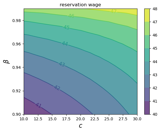
As expected, the reservation wage increases with both patience and unemployment compensation.
50.4. Computing an Optimal Policy: Take 2#
The approach to dynamic programming just described is standard and broadly applicable.
But for our McCall search model there’s also an easier way that circumvents the need to compute the value function.
Let \(h\) denote the continuation value:
The Bellman equation can now be written as
Now let’s derive a nonlinear equation for \(h\) alone.
Starting from (50.9), we multiply both sides by \(q(w')\) to get
Next, we sum both sides over \(w' \in \mathbb{W}\):
Now multiply both sides by \(\beta\):
Add \(c\) to both sides:
Finally, using the definition of \(h\) from (50.8), the left-hand side is just \(h\), giving us
This is a nonlinear equation in the single scalar \(h\) that we can solve for \(h\).
As before, we will use successive approximations:
Step 1: pick an initial guess \(h\).
Step 2: compute the update \(h'\) via
Step 3: calculate the deviation \(|h - h'|\).
Step 4: if the deviation is larger than some fixed tolerance, set \(h = h'\) and go to step 2, else return \(h\).
One can again use the Banach contraction mapping theorem to show that this process always converges.
The big difference here, however, is that we’re iterating on a scalar \(h\), rather than an \(n\)-vector, \(v(i), i = 1, \ldots, n\).
Here’s an implementation:
def compute_reservation_wage_two(
        model: McCallModel,   # instance containing default parameters
        tol: float=1e-5,      # error tolerance
        max_iter: int=500,    # maximum number of iterations for loop
    ):
    c, β, w, q = model
    h = (w @ q) / (1 - β)  # initial condition
    i = 0
    error = tol + 1
    initial_loop_state = i, h, error

    def cond(loop_state):
        i, h, error = loop_state
        return jnp.logical_and(i < max_iter, error > tol)

    def update(loop_state):
        i, h, error = loop_state
        s = jnp.maximum(w / (1 - β), h)
        h_next = c + β * (s @ q)
        error = jnp.abs(h_next - h)
        i_next = i + 1
        new_loop_state = i_next, h_next, error
        return new_loop_state

    final_state = jax.lax.while_loop(cond, update, initial_loop_state)
    i, h, error = final_state

    # Compute and return the reservation wage
    return (1 - β) * h
You can use this code to solve the exercise below.
50.5. Continuous Offer Distribution#
The discrete wage offer distribution used above is convenient for theory and computation, but many realistic distributions are continuous (i.e., have a density).
Fortunately, the theory changes little in our simple model when we shift to a continuous offer distribution.
Recall that \(h\) in (50.8) denotes the value of not accepting a job in this period but then behaving optimally in all subsequent periods.
To shift to a continuous offer distribution, we can replace (50.8) by
Equation (50.10) becomes
The aim is to solve this nonlinear equation by iteration, and from it obtain the reservation wage.
50.5.1. Implementation with Lognormal Wages#
Let’s implement this for the case where
the state sequence \(\{ s_t \}\) is IID and standard normal and
the wage function is \(w(s) = \exp(\mu + \sigma s)\).
This gives us a lognormal wage distribution.
We use Monte Carlo integration to evaluate the integral, averaging over a large number of wage draws.
For default parameters, we use c=25, β=0.99, σ=0.5, μ=2.5.
class McCallModelContinuous(NamedTuple):
    c: float              # unemployment compensation
    β: float              # discount factor
    σ: float              # scale parameter in lognormal distribution
    μ: float              # location parameter in lognormal distribution
    w_draws: jnp.ndarray  # draws of wages for Monte Carlo


def create_mccall_continuous(
        c=25, β=0.99, σ=0.5, μ=2.5, mc_size=1000, seed=1234
    ):
    key = jax.random.PRNGKey(seed)
    s = jax.random.normal(key, (mc_size,))
    w_draws = jnp.exp(μ + σ * s)
    return McCallModelContinuous(c, β, σ, μ, w_draws)


@jax.jit
def compute_reservation_wage_continuous(model, max_iter=500, tol=1e-5):
    c, β, σ, μ, w_draws = model

    h = jnp.mean(w_draws) / (1 - β)  # initial guess

    def update(state):
        h, i, error = state
        integral = jnp.mean(jnp.maximum(w_draws / (1 - β), h))
        h_next = c + β * integral
        error = jnp.abs(h_next - h)
        return h_next, i + 1, error

    def cond(state):
        h, i, error = state
        return jnp.logical_and(i < max_iter, error > tol)

    initial_state = (h, 0, tol + 1)
    final_state = jax.lax.while_loop(cond, update, initial_state)
    h_final, _, _ = final_state

    # Now compute the reservation wage
    return (1 - β) * h_final
Now let’s investigate how the reservation wage changes with \(c\) and \(\beta\) using a contour plot.
grid_size = 25
c_vals = jnp.linspace(10.0, 30.0, grid_size)
β_vals = jnp.linspace(0.9, 0.99, grid_size)

def compute_R_element(c, β):
    model = create_mccall_continuous(c=c, β=β)
    return compute_reservation_wage_continuous(model)

# First, vectorize over β (holding c fixed)
compute_R_over_β = jax.vmap(compute_R_element, in_axes=(None, 0))

# Next, vectorize over c (applying the above function to each c)
compute_R_vectorized = jax.vmap(compute_R_over_β, in_axes=(0, None))

# Apply to compute the full grid
R = compute_R_vectorized(c_vals, β_vals)
fig, ax = plt.subplots()

cs1 = ax.contourf(c_vals, β_vals, R.T, alpha=0.75)
ctr1 = ax.contour(c_vals, β_vals, R.T)

plt.clabel(ctr1, inline=1, fontsize=13)
plt.colorbar(cs1, ax=ax)


ax.set_title("reservation wage")
ax.set_xlabel("$c$", fontsize=16)
ax.set_ylabel("$β$", fontsize=16)

ax.ticklabel_format(useOffset=False)

plt.show()
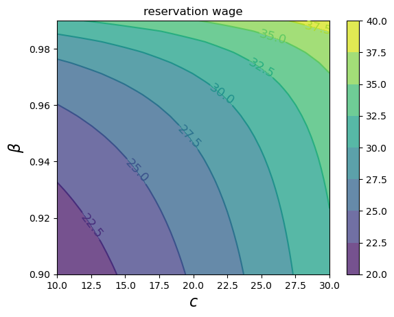
As with the discrete case, the reservation wage increases with both patience and unemployment compensation.
50.6. Volatility#
An interesting feature of the McCall model is that increased volatility in wage offers tends to increase the reservation wage.
The intuition is that volatility is attractive to the worker because they can enjoy the upside (high wage offers) while rejecting the downside (low wage offers).
Hence, with more volatility, workers are more willing to continue searching rather than accept a given offer, which means the reservation wage rises.
To illustrate this phenomenon, we use a mean-preserving spread of the wage distribution.
In particular, we vary the scale parameter \(\sigma\) in the lognormal wage distribution \(w(s) = \exp(\mu + \sigma s)\) while adjusting \(\mu\) to keep the mean constant.
Recall that for a lognormal distribution with parameters \(\mu\) and \(\sigma\), the mean is \(\exp(\mu + \sigma^2/2)\).
To keep the mean constant at some value \(m\), we need:
Let’s implement this and compute the reservation wage for different values of \(\sigma\):
# Fix the mean wage
mean_wage = 20.0

# Create a range of volatility values
σ_vals = jnp.linspace(0.1, 1.0, 25)

# Given σ, compute μ to maintain constant mean
def compute_μ_for_mean(σ, mean_wage):
    return jnp.log(mean_wage) - (σ**2) / 2

# Compute reservation wage for each volatility level
res_wages_volatility = []

for σ in σ_vals:
    μ = compute_μ_for_mean(σ, mean_wage)
    model = create_mccall_continuous(σ=float(σ), μ=float(μ))
    w_bar = compute_reservation_wage_continuous(model)
    res_wages_volatility.append(w_bar)

res_wages_volatility = jnp.array(res_wages_volatility)
Now let’s plot the reservation wage as a function of volatility:
fig, ax = plt.subplots()
ax.plot(σ_vals, res_wages_volatility, linewidth=2)
ax.set_xlabel(r'volatility ($\sigma$)', fontsize=12)
ax.set_ylabel('reservation wage', fontsize=12)
plt.show()
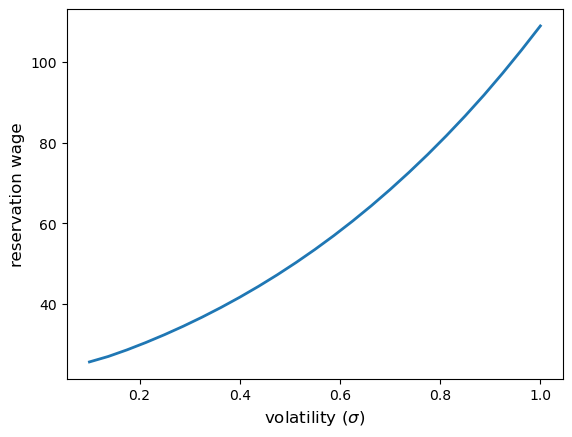
As expected, the reservation wage is increasing in \(\sigma\).
50.6.1. Lifetime Value and Volatility#
We’ve seen that the reservation wage increases with volatility.
It’s also the case that maximal lifetime value increases with volatility.
Higher volatility provides more upside potential, while at the same time workers can protect themselves against downside risk by rejecting low offers.
This option value translates into higher expected lifetime utility.
To demonstrate this, we will:
Compute the reservation wage for each volatility level
Calculate the expected discounted value of the lifetime income stream associated with that reservation wage, using Monte Carlo.
The simulation works as follows:
Compute the present discounted value of one lifetime earnings path, from a given wage path.
Average over a large number of such calculations to approximate expected discounted value.
We truncate each path at \(T=100\), which provides sufficient resolution for our purposes.
@jax.jit
def simulate_lifetime_value(key, model, w_bar, n_periods=100):
    """
    Simulate one realization of the wage path and compute lifetime value.

    Parameters:
    -----------
    key : jax.random.PRNGKey
        Random key for JAX
    model : McCallModelContinuous
        The model containing parameters
    w_bar : float
        The reservation wage
    n_periods : int
        Number of periods to simulate

    Returns:
    --------
    lifetime_value : float
        Discounted sum of income over n_periods
    """
    c, β, σ, μ, w_draws = model

    # Draw all wage offers upfront
    key, subkey = jax.random.split(key)
    s_vals = jax.random.normal(subkey, (n_periods,))
    wage_offers = jnp.exp(μ + σ * s_vals)

    # Determine which offers are acceptable
    accept = wage_offers >= w_bar

    # Track employment status: employed from first acceptance onward
    employed = jnp.cumsum(accept) > 0

    # Get the accepted wage (first wage where accept is True)
    first_accept_idx = jnp.argmax(accept)
    accepted_wage = wage_offers[first_accept_idx]

    # Earnings at each period: accepted_wage if employed, c if unemployed
    earnings = jnp.where(employed, accepted_wage, c)

    # Compute discounted sum
    periods = jnp.arange(n_periods)
    discount_factors = β ** periods
    lifetime_value = jnp.sum(discount_factors * earnings)

    return lifetime_value


@jax.jit
def compute_mean_lifetime_value(model, w_bar, num_reps=10000, seed=1234):
    """
    Compute mean lifetime value across many simulations.

    """
    key = jax.random.PRNGKey(seed)
    keys = jax.random.split(key, num_reps)

    # Vectorize the simulation across all replications
    simulate_fn = jax.vmap(simulate_lifetime_value, in_axes=(0, None, None))
    lifetime_values = simulate_fn(keys, model, w_bar)
    return jnp.mean(lifetime_values)
Now let’s compute the expected lifetime value for each volatility level:
# Use the same volatility range and mean wage
σ_vals = jnp.linspace(0.1, 1.0, 25)
mean_wage = 20.0

lifetime_vals = []
for σ in σ_vals:
    μ = compute_μ_for_mean(σ, mean_wage)
    model = create_mccall_continuous(σ=σ, μ=μ)
    w_bar = compute_reservation_wage_continuous(model)
    lv = compute_mean_lifetime_value(model, w_bar)
    lifetime_vals.append(lv)
Let’s visualize the expected lifetime value as a function of volatility:
fig, ax = plt.subplots()
ax.plot(σ_vals, lifetime_vals, linewidth=2, color='green')
ax.set_xlabel(r'volatility ($\sigma$)', fontsize=12)
ax.set_ylabel('expected lifetime value', fontsize=12)
plt.show()
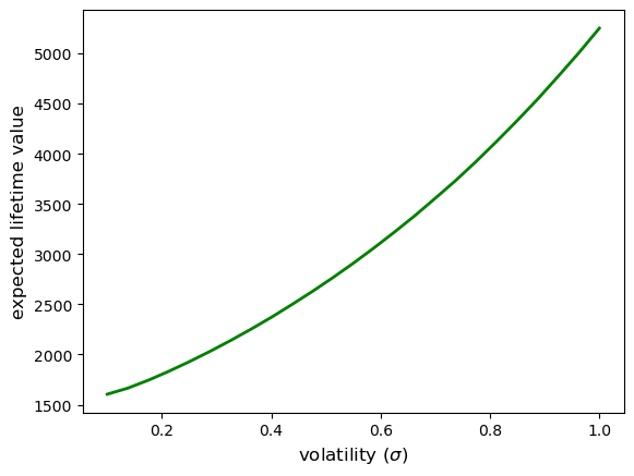
The plot confirms that despite workers setting higher reservation wages when facing more volatile wage offers (as shown above), they achieve higher expected lifetime values due to the option value of search.
50.7. Exercises#
Exercise 50.1
Compute the average duration of unemployment when \(\beta=0.99\) and \(c\) takes the following values
c_vals = np.linspace(10, 40, 4)
That is, start the agent off as unemployed, compute their reservation wage given the parameters, and then simulate to see how long it takes to accept.
Repeat a large number of times and take the average.
Plot mean unemployment duration as a function of \(c\) in c_vals.
Try to explain what you see.
Solution
Here’s a solution using the continuous wage offer distribution with JAX.
def compute_stopping_time_continuous(w_bar, key, model):
    """
    Compute stopping time by drawing wages from the continuous distribution
    until one exceeds `w_bar`.

    Parameters:
    -----------
    w_bar : float
        The reservation wage
    key : jax.random.PRNGKey
        Random key for JAX
    model : McCallModelContinuous
        The model containing wage draws

    Returns:
    --------
    t_final : int
        The stopping time (number of periods until acceptance)
    """
    c, β, σ, μ, w_draws = model

    def update(loop_state):
        t, key, accept = loop_state
        key, subkey = jax.random.split(key)
        # Draw a standard normal and transform to wage
        s = jax.random.normal(subkey)
        w = jnp.exp(μ + σ * s)
        accept = w >= w_bar
        t = t + 1
        return t, key, accept

    def cond(loop_state):
        _, _, accept = loop_state
        return jnp.logical_not(accept)

    initial_loop_state = (0, key, False)
    t_final, _, _ = jax.lax.while_loop(cond, update, initial_loop_state)
    return t_final


def compute_mean_stopping_time_continuous(w_bar, model, num_reps=100000, seed=1234):
    """
    Generate a mean stopping time over `num_reps` repetitions.

    Parameters:
    -----------
    w_bar : float
        The reservation wage
    model : McCallModelContinuous
        The model containing parameters
    num_reps : int
        Number of simulation replications
    seed : int
        Random seed

    Returns:
    --------
    mean_time : float
        Average stopping time across all replications
    """
    # Generate a key for each MC replication
    key = jax.random.PRNGKey(seed)
    keys = jax.random.split(key, num_reps)

    # Vectorize compute_stopping_time_continuous and evaluate across keys
    compute_fn = jax.vmap(compute_stopping_time_continuous, in_axes=(None, 0, None))
    obs = compute_fn(w_bar, keys, model)

    # Return mean stopping time
    return jnp.mean(obs)


# Compute mean stopping time for different values of c
c_vals = jnp.linspace(10, 40, 4)

@jax.jit
def compute_stop_time_for_c_continuous(c):
    """Compute mean stopping time for a given compensation value c."""
    model = create_mccall_continuous(c=c)
    w_bar = compute_reservation_wage_continuous(model)
    return compute_mean_stopping_time_continuous(w_bar, model)

# Vectorize across all c values
compute_stop_time_vectorized = jax.vmap(compute_stop_time_for_c_continuous)
stop_times = compute_stop_time_vectorized(c_vals)

fig, ax = plt.subplots()

ax.plot(c_vals, stop_times, label="mean unemployment duration")
ax.set(xlabel="unemployment compensation", ylabel="months")
ax.legend()

plt.show()