113. Asymmetry and Large Shocks in Unemployment#
GPU
This lecture was built using a machine with access to a GPU — although it will also run without one.
Google Colab has a free tier with GPUs that you can access as follows:
Click on the “play” icon top right
Select Colab
Set the runtime environment to include a GPU
In addition to what’s in Anaconda, this lecture needs the following libraries.
We first install numpyro and jax:
!pip install numpyro jax
We also install pandas_datareader, which we use to download data from FRED:
!pip install pandas_datareader
We also use ArviZ for model comparison:
!pip install arviz
113.1. Overview#
This lecture is a sequel to A Linear Model of Unemployment.
There we fit a linear AR(1) model to the US unemployment rate and examined persistence.
One thing we found but didn’t address is that the model’s residuals were both heavy-tailed and right-skewed.
Unemployment jumps up sharply in recessions and drifts down slowly in recoveries.
A model with symmetric Gaussian shocks cannot reproduce these features.
In this lecture we allow the innovations to be right-skewed and, to some degree, heavy-tailed.
We also use this lecture to develop a very useful Bayesian technique: model comparison by leave-one-out cross-validation.
We use this to decide whether one model really predicts better than another.
Our plan is to
build a model with a linear mean but asymmetric, occasionally-large shocks,
estimate it on the annual data,
compare it to the original Gaussian model with cross-validation, and
check whether it captures the asymmetry the original model missed.
Let’s start with some imports.
import numpy as np
import matplotlib.pyplot as plt
import datetime as dt
from pandas_datareader import data as web

import jax.numpy as jnp
from jax import random
import numpyro
import numpyro.distributions as dist
from numpyro.infer import MCMC, NUTS, log_likelihood
113.2. The data#
We use the same series as in A Linear Model of Unemployment — the US unemployment rate (UNRATE from FRED), excluding the COVID-19 spike — and work at an annual frequency, where the recessions stand out as clean spikes.
start, end = dt.datetime(1948, 1, 1), dt.datetime(2024, 12, 31)
unrate = web.DataReader("UNRATE", "fred", start, end)["UNRATE"]
pre_covid = unrate[unrate.index < "2020-01-01"]
u_annual = pre_covid.resample("YE").last().to_numpy()
years = pre_covid.resample("YE").last().index.year
The shape we want to capture is plain in the annual series.
fig, ax = plt.subplots()
ax.plot(years, u_annual, lw=2, marker='o', ms=3)
ax.set_xlabel('year')
ax.set_ylabel('unemployment rate (%)')
plt.show()
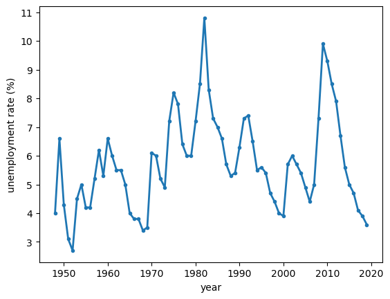
Fig. 113.1 Annual US unemployment#
In Fig. 113.1 each recession is a sharp rise followed by a long, gradual decline — fast up, slow down.
113.3. A model with asymmetric shocks#
We keep the linear reversion of A Linear Model of Unemployment and change only the shock:
where the innovation \(\eta_{t+1}\) is drawn from a mixture of two normals:
The model has six parameters:
symbol |
name |
role |
|---|---|---|
\(\bar u\) |
floor |
the low level the series reverts to |
\(\rho\) |
persistence |
speed of reversion (as in the linear lecture) |
\(p\) |
jump probability |
how often a large shock arrives |
\(\mu_J\) |
jump size |
the average upward kick of a recession |
\(\sigma_s,\ \sigma_J\) |
shock spreads |
the quiet and jumpy volatilities |
The mechanism leads to a sawtooth dynamic for the unemployment rate.
Most years are quiet, with small noise; occasionally a positive jump throws unemployment up; then, with no further jumps, the linear reversion \(\rho\) glides it slowly back down toward \(\bar u\).
A spike arrives in one step, the recovery takes many — fast up, slow down.
Because \(\rho < 1\) the series is still stationary and bounded.
All that has changed is that the shocks can be large and one-sided.
This is, in spirit, Milton Friedman’s “plucking” picture: a floor near full employment, from which recessions pluck the series upward.
The next cell draws an illustrative innovation density and its two components.
def normal_pdf(x, m, s):
    return np.exp(-(x - m)**2 / (2 * s**2)) / (s * np.sqrt(2 * np.pi))

η = np.linspace(-3, 6, 400)
p_, μJ_, σs_, σJ_ = 0.25, 2.0, 0.4, 1.2
quiet = (1 - p_) * normal_pdf(η, 0.0, σs_)
jump  = p_ * normal_pdf(η, μJ_, σJ_)

fig, ax = plt.subplots()
ax.plot(η, quiet + jump, lw=2, label='shock density')
ax.fill_between(η, quiet, alpha=0.3, label='quiet years')
ax.fill_between(η, jump, alpha=0.3, label='recession jumps')
ax.set_xlabel('innovation $\\eta$')
ax.legend()
plt.show()
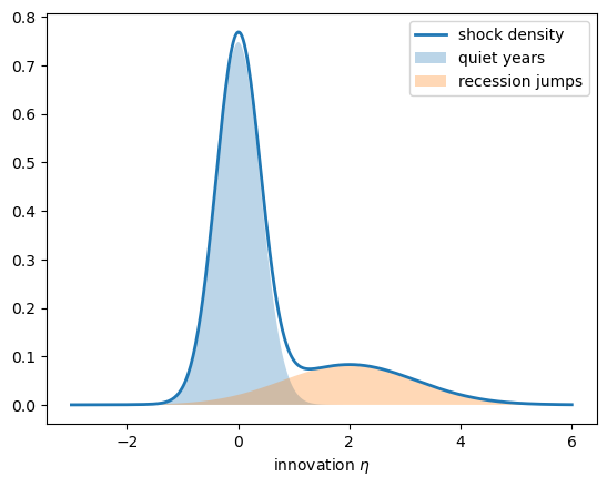
Fig. 113.2 The two-component shock distribution#
Fig. 113.2 shows the signature shape: a tall, narrow peak at zero for ordinary years, plus a low, broad bump on the positive side for the recession jumps.
That right-leaning bump is what the symmetric Gaussian of the linear lecture cannot produce.
113.4. Bayesian estimation#
We place weakly informative priors on the six parameters, anchoring \(\bar u\) low (a floor) and making jumps occasional.
The mixture is written with NumPyro’s MixtureSameFamily, which sums over the two components analytically — so there is no discrete “which component?” variable for the sampler to struggle with.
def jump_model(u):
    ubar = numpyro.sample("ubar",    dist.Normal(4.5, 1.5))
    ρ    = numpyro.sample("rho",     dist.Uniform(0.0, 1.0))
    p    = numpyro.sample("p",       dist.Beta(2.0, 8.0))
    μ_J  = numpyro.sample("mu_J",    dist.HalfNormal(2.0))
    σ_s  = numpyro.sample("sigma_s", dist.HalfNormal(0.5))
    σ_J  = numpyro.sample("sigma_J", dist.HalfNormal(1.5))
    n = u.shape[0] - 1
    base   = ubar + ρ * (u[:-1] - ubar)
    locs   = jnp.stack([base, base + μ_J], axis=-1)
    scales = jnp.stack([jnp.broadcast_to(σ_s, (n,)),
                        jnp.broadcast_to(σ_J, (n,))], axis=-1)
    probs  = jnp.broadcast_to(jnp.stack([1 - p, p]), (n, 2))
    mix = dist.MixtureSameFamily(dist.Categorical(probs=probs),
                                 dist.Normal(locs, scales))
    numpyro.sample("u_obs", mix, obs=u[1:])
We sample with NUTS, four chains, vectorized so the code runs on a CPU or a GPU.
def run_nuts(model, data, seed=0, num_warmup=2000, num_samples=4000, num_chains=4):
    "Sample a NumPyro model with the NUTS sampler."
    mcmc = MCMC(NUTS(model),
                num_warmup=num_warmup, num_samples=num_samples,
                num_chains=num_chains, chain_method="vectorized",
                progress_bar=False)
    mcmc.run(random.PRNGKey(seed), jnp.asarray(data))
    return mcmc
We fit the model to the annual data.
mcmc_jump = run_nuts(jump_model, u_annual)
Let us look at the posterior.
mcmc_jump.print_summary()
                mean       std    median      5.0%     95.0%     n_eff     r_hat
      mu_J      1.26      0.43      1.20      0.57      2.00   3583.57      1.00
         p      0.35      0.09      0.35      0.19      0.49   4178.84      1.00
       rho      0.83      0.04      0.84      0.76      0.90   5632.75      1.00
   sigma_J      1.28      0.26      1.29      0.83      1.73   3970.18      1.00
   sigma_s      0.39      0.09      0.38      0.25      0.54   3715.71      1.00
      ubar      3.03      0.74      3.09      1.81      4.19   5156.56      1.00

Number of divergences: 0
The r_hat values are essentially one, so the chains have converged.
The estimates tell a coherent story:
a floor \(\bar u\) around 3%
slow reversion (\(\rho \approx 0.8\)), and
a distinct jump component: the quiet spread \(\sigma_s\) is small and the jump spread \(\sigma_J\) is several times larger, with a positive mean \(\mu_J\).
The data have split the innovations into “ordinary years” and “recession years” on their own.
We can see that split by overlaying the fitted shock density on the model’s actual residuals.
m = {k: np.median(np.asarray(mcmc_jump.get_samples()[k]))
     for k in ("ubar", "rho", "p", "mu_J", "sigma_s", "sigma_J")}
resid = u_annual[1:] - (m["ubar"] + m["rho"] * (u_annual[:-1] - m["ubar"]))

η = np.linspace(resid.min() - 0.5, resid.max() + 0.5, 400)
quiet = (1 - m["p"]) * normal_pdf(η, 0.0, m["sigma_s"])
jump  = m["p"] * normal_pdf(η, m["mu_J"], m["sigma_J"])

fig, ax = plt.subplots()
ax.hist(resid, bins=25, density=True, alpha=0.5, label='residuals')
ax.plot(η, quiet + jump, lw=2, label='fitted density')
ax.fill_between(η, jump, alpha=0.3, color='C2', label='jump component')
ax.set_xlabel('innovation $\\eta$')
ax.legend()
plt.show()
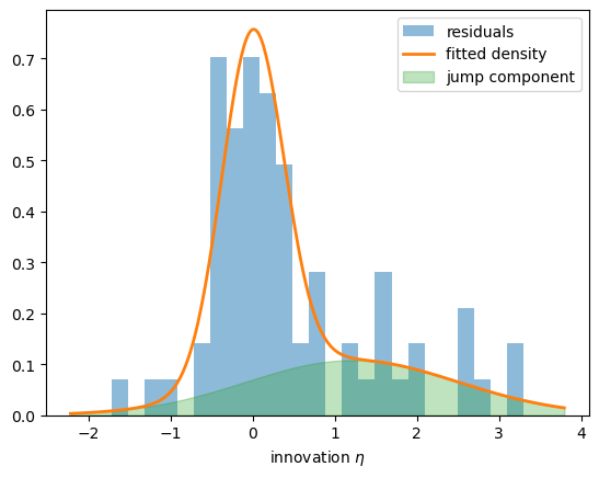
Fig. 113.3 Fitted shock density against the residuals#
In Fig. 113.3 the fitted density tracks the residuals, with the jump component accounting for the spread of large positive surprises on the right.
113.5. Comparing models with cross-validation#
The jump model looks reasonable, but is it actually better than the linear one?
To answer this question, we will use Bayesian model comparison.
We build it up in stages: the guiding principle, the leave-one-out estimate, and how the computation is actually done.
113.5.1. The guiding principle: look at predictions, not in-sample fit#
It is tempting to compare two models by asking which one fits the observed data better.
This isn’t the right criterion: more complex models can always be tuned to better match the data they are fitting.
The right question is instead: which model better predicts data it has not seen?
In other words, the criterion we care about is out-of-sample predictive accuracy.
113.5.2. Leave-one-out cross-validation#
We do not have new data, so we create some by cross-validation.
The idea is to leave out one observation, fit the model to the rest, and then score the held-out point using a predictive distribution constructed from the rest of the data set.
The predictive distribution for data point \(u_i\) given the rest of the data \(u_{-i}\) is
We score each held-out point by the log of this density: the logarithm rewards a model for putting high probability on what actually happened, and it makes the scores for the whole data set add up rather than multiply.
Adding these scores gives the expected log predictive density (elpd), here in its leave-one-out (LOO) form,
113.5.3. Computing it from a single fit#
If we calculate this measure naively, we need to refit the model \(n\) times, once for each omitted point, which is very time consuming.
The trick that makes LOO practical is that we can avoid all but the first fit, by reweighting the posterior we already have.
Start from the quantity we want, which is an expectation over the leave-one-out posterior:
We do not have draws from \(p(\theta \mid u_{-i})\), but we do have \(S\) draws \(\theta^1, \dots, \theta^S\) from the full posterior \(p(\theta \mid u)\) — the chains we already ran.
The two posteriors differ by a single factor.
The likelihood is a product of one per-observation term, so dropping observation \(i\) just removes its factor:
where the last step uses \(p(\theta \mid u) \propto p(\theta) \prod_j p(u_j \mid \theta)\).
A draw from the full posterior can therefore stand in for the leave-\(i\)-out posterior if we give it the importance weight
which downweights exactly the draws that fit \(u_i\) well, since their good fit to \(u_i\) is the influence we want to remove.
Estimating the expectation by self-normalized importance sampling, and then substituting this weight, the numerator collapses because \(w_i^s\, p(u_i \mid \theta^s) = 1\):
The right-hand side is the harmonic mean of the per-draw likelihoods of \(u_i\), with \(S\) the number of posterior draws.
Its only ingredient is the likelihood of each observation under each posterior draw — the pointwise log-likelihood — which is why, throughout, we have been careful to compute it.
In code we work on the log scale for stability, where the harmonic mean becomes
which is the np.log(S) - logsumexp(-ll) we use below.
To compare against the linear model, we first fit it on the same data.
def linear_model(u):
    ubar = numpyro.sample("ubar",  dist.Normal(5.5, 2.0))
    ρ    = numpyro.sample("rho",   dist.Uniform(0.0, 1.0))
    σ    = numpyro.sample("sigma", dist.HalfNormal(1.0))
    numpyro.sample("u_obs", dist.Normal(ubar + ρ * (u[:-1] - ubar), σ), obs=u[1:])
We sample it on the same annual data.
mcmc_lin = run_nuts(linear_model, u_annual)
Now we can do the whole leave-one-out calculation by hand in a few lines.
from scipy.special import logsumexp

def pointwise_loo(mcmc, model):
    "Leave-one-out log predictive density for each observation."
    ll = np.asarray(log_likelihood(model, mcmc.get_samples(),
                                   u=jnp.asarray(u_annual))["u_obs"])  # (draws, obs)
    S = ll.shape[0]
    # log of the harmonic mean of the per-draw likelihoods, per observation
    return np.log(S) - logsumexp(-ll, axis=0)

elpd_jump = pointwise_loo(mcmc_jump, jump_model)
elpd_lin  = pointwise_loo(mcmc_lin,  linear_model)

print(f"jump   elpd_loo = {elpd_jump.sum():.1f}")
print(f"linear elpd_loo = {elpd_lin.sum():.1f}")
jump   elpd_loo = -93.9
linear elpd_loo = -105.7
The jump model scores higher (closer to zero), so on out-of-sample prediction it wins.
To judge whether the gap is real, we need its uncertainty.
Because the total elpd is a sum over observations, the difference between the two models is itself a sum of per-observation differences, and its standard error follows from their spread.
diff = elpd_jump - elpd_lin
n = diff.size
print(f"elpd difference = {diff.sum():.1f}")
print(f"standard error  = {np.sqrt(n) * diff.std():.1f}")
elpd difference = 11.8
standard error  = 5.7
The jump model is ahead by about twelve points, against a standard error near six — a bit over two standard errors, so a real improvement and not a fluke.
113.5.4. Letting ArviZ do it#
In practice we let a library handle the bookkeeping, and add two refinements.
The raw importance weights \(1/p(u_i\mid\theta^s)\) can occasionally be dominated by a single extreme draw; ArviZ stabilizes them with Pareto-smoothed importance sampling, and reports a diagnostic — the Pareto shape \(\hat k\) — that flags any observation where the estimate is unreliable (a value above \(0.7\) is the usual warning line).
We hand it the same pointwise log-likelihoods, packaged in its data format.
import arviz as az
import xarray as xr

def to_arviz(mcmc, model, u):
    "Package a NumPyro fit for ArviZ, with pointwise log-likelihoods."
    idata = az.from_numpyro(mcmc)
    ll = np.asarray(log_likelihood(model, mcmc.get_samples(),
                                   u=jnp.asarray(u))["u_obs"])
    ll = ll.reshape(mcmc.num_chains, -1, ll.shape[-1])
    idata["log_likelihood"] = xr.Dataset(
        {"u_obs": (("chain", "draw", "obs"), ll)})
    return idata

az.compare({
    "linear": to_arviz(mcmc_lin,  linear_model, u_annual),
    "jump":   to_arviz(mcmc_jump, jump_model,   u_annual),
})
| rank | elpd_diff | dse | p_worse | diag_diff | diag_elpd | p | elpd | se | weight | |
|---|---|---|---|---|---|---|---|---|---|---|
| jump | 0 | 0.0 | 0.0 | NaN | 6.5 | -90.0 | 9.2 | 0.87 | ||
| linear | 1 | -10.0 | 5.7 | 0.98 | N < 100 | 3.6 | -110.0 | 7.3 | 0.13 |
Here the smoothing changes nothing — every \(\hat k\) stays below \(0.7\) — so az.compare confirms the hand calculation and ranks the jump model first (its table rounds the scores for display).
113.5.5. Reading the comparison#
Two of the columns repay a closer look.
The column p is the effective number of parameters: not the count we wrote down, but how much freedom the data actually grant the model, estimated from the gap between its in-sample and out-of-sample fit.
It is about three and a half for the linear model and six and a half for the jump model — and, tellingly, it need not equal the nominal parameter count, since a parameter the data cannot pin down adds almost nothing to it.
Readers from classical statistics will recognize the whole exercise: it is the goal behind the AIC, which estimates out-of-sample accuracy as in-sample fit minus a parameter count.
LOO reaches that goal without the asymptotic shortcut — it uses the entire posterior and learns the effective complexity from the data.
(The BIC, by contrast, aims at a different target, the marginal likelihood, and hence the probability that each model is true; that is the province of Bayes factors, not of predictive accuracy.)
Finally, a word of caution: these standard errors rest on only about seventy observations, so they are rough.
There is also a deeper issue, special to time series, which we take up now.
113.5.6. Accommodating the time series structure#
Leave-one-out drops one transition at a time, but it does not respect the order of time.
When it scores the step from \(u_t\) to \(u_{t+1}\), the model doing the scoring was fit on data lying on both sides of that step — including the neighboring values \(u_t\) and \(u_{t+1}\) themselves.
So the held-out point was never truly unseen, and a time series, unlike an exchangeable sample, has an arrow of time that this ignores.
The formally correct measure is leave-future-out cross-validation.
It only ever predicts forward: fit the model on \(u_1, \dots, u_t\), score its one-step-ahead forecast of \(u_{t+1}\), then expand the window by one step and repeat.
Now the model is genuinely blind to the future it is asked to predict, exactly as in real forecasting.
The price is computational.
Leave-one-out reused a single fit through its importance-sampling shortcut, but leave-future-out has no such trick — each step conditions on a different stretch of history, so the model must be refit from scratch, dozens of times rather than once.
For our short annual series that is minutes rather than seconds; for a long series it can become prohibitive.
We ran it anyway, and the conclusion holds: under leave-future-out the jump model still beats the linear one, by an even clearer margin than leave-one-out reported.
Genuine forecasting favors the asymmetric shocks more strongly, not less — so the verdict survives the stricter test.
113.6. Does it capture the asymmetry?#
LOO says the jump model predicts better, but we built it for a specific reason: to reproduce the asymmetry.
A posterior predictive check tests exactly that.
We pick a statistic that summarizes the asymmetry — the skewness of the annual changes \(\Delta u\) — and ask whether paths simulated from the fitted model produce values like the one we see in the data.
A symmetric model is pinned at a skewness of zero and cannot pass; the jump model should.
def simulate(u0, T, ubar, ρ, p, μ_J, σ_s, σ_J, rng):
    "Simulate a path of the jump model."
    u = np.empty(T)
    u[0] = u0
    for t in range(1, T):
        η = rng.normal(μ_J, σ_J) if rng.random() < p else rng.normal(0.0, σ_s)
        u[t] = ubar + ρ * (u[t-1] - ubar) + η
    return u

def skewness(x):
    x = x - x.mean()
    return (x**3).mean() / x.std()**3

post = mcmc_jump.get_samples()
keys = ("ubar", "rho", "p", "mu_J", "sigma_s", "sigma_J")
draws = {k: np.asarray(post[k]) for k in keys}

rng = np.random.default_rng(1)
T, N = len(u_annual), 2000
idx = rng.integers(0, len(draws["rho"]), N)
sims = np.array([simulate(u_annual[0], T, *(draws[k][i] for k in keys), rng)
                 for i in idx])

obs_skew = skewness(np.diff(u_annual))
rep_skew = np.array([skewness(np.diff(s)) for s in sims])
print(f"observed skewness of Δu = {obs_skew:.2f}")
print(f"posterior predictive P(skew > observed) = {(rep_skew > obs_skew).mean():.2f}")
observed skewness of Δu = 0.77
posterior predictive P(skew > observed) = 0.73
The observed annual changes are right-skewed, and the simulated paths reproduce that skew, with the observed value sitting comfortably inside the predictive distribution.
The figure makes the check, and the sawtooth, visible.
fig, (a0, a1, a2) = plt.subplots(1, 3, figsize=(15, 4.2))

lo, mid, hi = np.percentile(sims, [5, 50, 95], axis=0)
a0.fill_between(years, lo, hi, alpha=0.3, label='90% band')
a0.plot(years, u_annual, 'k', lw=2, label='observed')
a0.set_title('predictive band')
a0.set_xlabel('year')
a0.legend()

for s in sims[:6]:
    a1.plot(years, s, lw=1, alpha=0.7)
a1.plot(years, u_annual, 'k', lw=2.5, label='observed')
a1.set_title('simulated paths')
a1.set_xlabel('year')
a1.legend()

a2.hist(rep_skew, bins=50, density=True, alpha=0.6)
a2.axvline(obs_skew, color='k', lw=2, label='observed')
a2.set_title('skewness of $\\Delta u$')
a2.set_xlabel('skewness')
a2.legend()
plt.show()
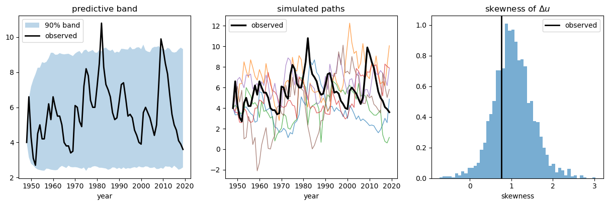
Fig. 113.4 Posterior predictive check for the asymmetry#
The left panel shows the observed series staying inside the predictive band; the middle panel shows simulated paths with the same spiky, fast-up-slow-down character as the data; and the right panel shows the observed skewness falling in the bulk of the predictive distribution.
The symmetric models of A Linear Model of Unemployment would put that vertical line far out in the tail.
113.7. Conclusion#
In A Linear Model of Unemployment we applied a linear AR(1) model with Gaussian shocks to unemployment and found a high levels of persistence in monthly data.
We also argued that the model is overly simplistic.
Here we found that the feature the linear model most conspicuously misses — the asymmetry of recessions — can be addressed by considering the distribution of the shocks.
A linear reversion with large, one-sided innovations reproduces the spikes, the slow recoveries, and the boundedness, and cross-validation prefers it clearly.
Along the way we learned about leave-one-out cross-validation, which helps us determine asks which model predicts better.
A richer model would let the economy switch between persistent expansion and recession regimes.
This is the Markov-switching approach of Hamilton, which we leave to further reading.
113.8. Exercises#
Exercise 113.1
The jump component here is symmetric within itself, \(N(\mu_J, \sigma_J^2)\).
Replace the two-component mixture with a single skew-normal (or Student-\(t\) with a skew) innovation, refit, and compare to the mixture model with az.compare.
Does the simpler skewed shock do as well as the mixture?