54. Job Search V: Persistent and Transitory Wage Shocks#
GPU
This lecture was built using a machine with access to a GPU — although it will also run without one.
Google Colab has a free tier with GPUs that you can access as follows:
Click on the “play” icon top right
Select Colab
Set the runtime environment to include a GPU
In addition to what’s in Anaconda, this lecture will need the following libraries:
!pip install quantecon jax
54.1. Overview#
In this lecture we extend the McCall job search model by decomposing wage offers into persistent and transitory components.
In the baseline model, wage offers are IID over time, which is unrealistic.
In Job Search III, we introduced correlated wage draws using a Markov chain, but we also added job separation.
Here we take a different approach: we model wage dynamics through an AR(1) process for the persistent component plus a transitory shock, while returning to the assumption that jobs are permanent (as in the baseline model).
This persistent-transitory decomposition is:
More realistic for modeling actual wage processes
Commonly used in labor economics (see, e.g., [MaCurdy, 1982], [Meghir and Pistaferri, 2004])
Simple enough to analyze while capturing key features of wage dynamics
By keeping jobs permanent, we can focus on understanding how persistent and transitory wage shocks affect search behavior and reservation wages.
We will solve the model using fitted value function iteration with linear interpolation, as introduced in Job Search IV.
We will use the following imports:
import matplotlib.pyplot as plt
import jax
import jax.numpy as jnp
import jax.random
import quantecon as qe
from typing import NamedTuple
54.2. The model#
Wages at each point in time are given by
where
Here \(\{ \zeta_t \}\) and \(\{ \epsilon_t \}\) are both IID and standard normal.
Here \(\{Y_t\}\) is a transitory component and \(\{Z_t\}\) is persistent.
As before, the worker can either
accept an offer and work permanently at that wage, or
take unemployment compensation \(c\) and wait till next period.
The value function satisfies the Bellman equation
In this expression, \(u\) is a utility function and \(\mathbb E_z\) is the expectation of next period variables given current \(z\).
The variable \(z\) enters as a state in the Bellman equation because its current value helps predict future wages.
54.2.1. A simplification#
There is a way that we can reduce dimensionality in this problem, which greatly accelerates computation.
To start, let \(f^*\) be the continuation value function, defined by
The Bellman equation can now be written
Combining the last two expressions, we see that the continuation value function satisfies
We’ll solve this functional equation for \(f^*\) by introducing the operator
By construction, \(f^*\) is a fixed point of \(Q\), in the sense that \(Q f^* = f^*\).
Under mild assumptions, it can be shown that \(Q\) is a contraction mapping over a suitable space of continuous functions on \(\mathbb R\).
By Banach’s contraction mapping theorem, this means that \(f^*\) is the unique fixed point and we can calculate it by iterating with \(Q\) from any reasonable initial condition.
Once we have \(f^*\), we can solve the search problem by stopping when the reward for accepting exceeds the continuation value, or
For utility, we take \(u(x) = \ln(x)\).
The reservation wage is the wage where equality holds in the last expression.
That is,
Our main aim is to solve for the reservation rule and study its properties and implications.
54.3. Implementation#
Let \(f\) be our initial guess of \(f^*\).
When we iterate, we use the fitted value function iteration algorithm.
In particular, \(f\) and all subsequent iterates are stored as a vector of values on a grid.
These points are interpolated into a function as required, using piecewise linear interpolation.
The integral in the definition of \(Qf\) is calculated by Monte Carlo.
Here’s a NamedTuple that stores the model parameters and data.
Default parameter values are embedded in the model.
class Model(NamedTuple):
    μ: float     # transient shock log mean
    s: float     # transient shock log variance
    d: float     # shift coefficient of persistent state
    ρ: float     # correlation coefficient of persistent state
    σ: float     # state volatility
    β: float     # discount factor
    c: float     # unemployment compensation
    z_grid: jnp.ndarray
    e_draws: jnp.ndarray

def create_job_search_model(μ=0.0, s=1.0, d=0.0, ρ=0.9, σ=0.1, β=0.98, c=5.0,
                           mc_size=1000, grid_size=100, key=jax.random.PRNGKey(1234)):
    """
    Create a Model with computed grid and draws.
    """
    # Set up grid
    z_mean = d / (1 - ρ)
    z_sd = σ / jnp.sqrt(1 - ρ**2)
    k = 3  # std devs from mean
    a, b = z_mean - k * z_sd, z_mean + k * z_sd
    z_grid = jnp.linspace(a, b, grid_size)

    # Draw and store shocks
    e_draws = jax.random.normal(key, (2, mc_size))

    return Model(μ, s, d, ρ, σ, β, c, z_grid, e_draws)
Next, we implement the \(Q\) operator.
def Q(model, f_in):
    """
    Apply the operator Q.

        * model is an instance of Model
        * f_in is an array that represents f
        * returns Qf

    """
    μ, s, d = model.μ, model.s, model.d
    ρ, σ, β, c = model.ρ, model.σ, model.β, model.c
    z_grid, e_draws = model.z_grid, model.e_draws
    M = e_draws.shape[1]

    def compute_expectation(z):
        def evaluate_shock(e):
            e1, e2 = e[0], e[1]
            z_next = d + ρ * z + σ * e1
            go_val = jnp.interp(z_next, z_grid, f_in)  # f(z')
            y_next = jnp.exp(μ + s * e2)               # y' draw
            w_next = jnp.exp(z_next) + y_next          # w' draw
            stop_val = jnp.log(w_next) / (1 - β)
            return jnp.maximum(stop_val, go_val)

        expectations = jax.vmap(evaluate_shock)(e_draws.T)
        return jnp.mean(expectations)

    expectations = jax.vmap(compute_expectation)(z_grid)
    f_out = jnp.log(c) + β * expectations
    return f_out
Here’s a function to compute an approximation to the fixed point of \(Q\).
@jax.jit
def compute_fixed_point(model, tol=1e-4, max_iter=1000):
    """
    Compute an approximation to the fixed point of Q.
    """

    def cond_fun(loop_state):
        f, i, error = loop_state
        return jnp.logical_and(error > tol, i < max_iter)

    def body_fun(loop_state):
        f, i, error = loop_state
        f_new = Q(model, f)
        error_new = jnp.max(jnp.abs(f_new - f))
        return f_new, i + 1, error_new

    # Initial state
    f_init = jnp.full(len(model.z_grid), jnp.log(model.c))
    init_state = (f_init, 0, tol + 1)

    # Run iteration
    f_final, iterations, final_error = jax.lax.while_loop(
        cond_fun, body_fun, init_state
    )

    return f_final
Let’s try generating an instance and solving the model.
model = create_job_search_model()

with qe.Timer():
    f_star = compute_fixed_point(model).block_until_ready()
0.4701 seconds elapsed
Next, we will compute and plot the reservation wage function defined in (54.1).
res_wage_function = jnp.exp(f_star * (1 - model.β))

fig, ax = plt.subplots()
ax.plot(
    model.z_grid, res_wage_function, label="reservation wage given $z$"
)
ax.set(xlabel="$z$", ylabel="wage")
ax.legend()
plt.show()
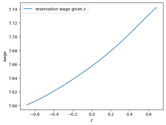
Notice that the reservation wage is increasing in the current state \(z\).
This is because a higher state leads the agent to predict higher future wages, increasing the option value of waiting.
Let’s try changing unemployment compensation and looking at its impact on the reservation wage:
c_vals = 1, 2, 3

fig, ax = plt.subplots()

for c in c_vals:
    model = create_job_search_model(c=c)
    f_star = compute_fixed_point(model)
    res_wage_function = jnp.exp(f_star * (1 - model.β))
    ax.plot(model.z_grid, res_wage_function,
                label=rf"$\bar w$ at $c = {c}$")

ax.set(xlabel="$z$", ylabel="wage")
ax.legend()
plt.show()
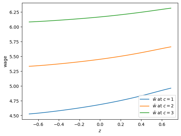
As expected, higher unemployment compensation shifts the reservation wage up at all state values.
54.4. Unemployment duration#
Next, we study how mean unemployment duration varies with unemployment compensation.
For simplicity, we’ll fix the initial state at \(Z_0 = 0\).
@jax.jit
def draw_duration(key, μ, s, d, ρ, σ, β, z_grid, f_star, t_max=10_000):
    """
    Draw unemployment duration for a single simulation.

    """
    def f_star_function(z):
        return jnp.interp(z, z_grid, f_star)

    def cond_fun(loop_state):
        z, t, unemployed, key = loop_state
        return jnp.logical_and(unemployed, t < t_max)

    def body_fun(loop_state):
        z, t, unemployed, key = loop_state
        key1, key2, key = jax.random.split(key, 3)

        # Draw current wage
        y = jnp.exp(μ + s * jax.random.normal(key1))
        w = jnp.exp(z) + y
        res_wage = jnp.exp(f_star_function(z) * (1 - β))

        # Check if optimal to stop
        accept = w >= res_wage
        τ = jnp.where(accept, t, t_max)

        # Update state if not accepting
        z_new = jnp.where(accept, z,
                            ρ * z + d + σ * jax.random.normal(key2))
        t_new = t + 1
        unemployed_new = jnp.logical_not(accept)

        return z_new, t_new, unemployed_new, key

    # Initial loop_state: (z, t, unemployed, key)
    init_state = (0.0, 0, True, key)
    z_final, t_final, unemployed_final, _ = jax.lax.while_loop(
        cond_fun, body_fun, init_state)

    # Return final time if job found, otherwise t_max
    return jnp.where(unemployed_final, t_max, t_final)


def compute_unemployment_duration(
        model, key=jax.random.PRNGKey(1234), num_reps=100_000
    ):
    """
    Compute expected unemployment duration.

    """
    f_star = compute_fixed_point(model)
    μ, s, d = model.μ, model.s, model.d
    ρ, σ, β = model.ρ, model.σ, model.β
    z_grid = model.z_grid

    # Generate keys for all simulations
    keys = jax.random.split(key, num_reps)

    # Vectorize over simulations
    τ_vals = jax.vmap(
        lambda k: draw_duration(k, μ, s, d, ρ, σ, β, z_grid, f_star)
    )(keys)

    return jnp.mean(τ_vals)
Let’s test this out with some possible values for unemployment compensation.
c_vals = jnp.linspace(1.0, 10.0, 8)
durations = []
for i, c in enumerate(c_vals):
    model = create_job_search_model(c=c)
    τ = compute_unemployment_duration(model, num_reps=10_000)
    durations.append(τ)
durations = jnp.array(durations)
Here is a plot of the results.
fig, ax = plt.subplots()
ax.plot(c_vals, durations)
ax.set_xlabel("unemployment compensation")
ax.set_ylabel("mean unemployment duration")
plt.show()
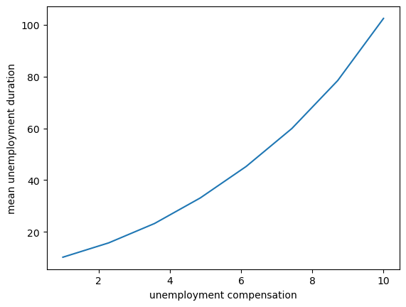
Not surprisingly, unemployment duration increases when unemployment compensation is higher.
This is because the value of waiting increases with unemployment compensation.
54.5. Exercises#
Exercise 54.1
Investigate how mean unemployment duration varies with the discount factor \(\beta\).
What is your prior expectation?
Do your results match up?
Solution
Here is one solution:
beta_vals = jnp.linspace(0.94, 0.99, 8)
durations = []
for i, β in enumerate(beta_vals):
    model = create_job_search_model(β=β)
    τ = compute_unemployment_duration(model, num_reps=10_000)
    durations.append(τ)
durations = jnp.array(durations)
fig, ax = plt.subplots()
ax.plot(beta_vals, durations)
ax.set_xlabel(r"$\beta$")
ax.set_ylabel("mean unemployment duration")
plt.show()
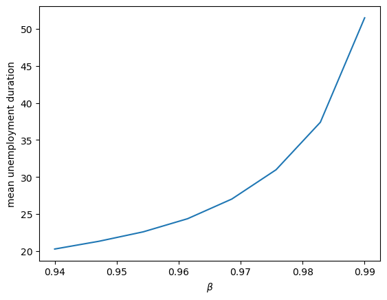
The figure shows that more patient individuals tend to wait longer before accepting an offer.