104. Speculative Behavior with Bayesian Learning#
104.1. Overview#
This lecture describes how Morris [1996] extended the Harrison–Kreps model [Harrison and Kreps, 1978] of speculative asset pricing.
Like Harrison and Kreps’s model, Morris’s model determines the price of a dividend-yielding asset that is traded by risk-neutral investors who have heterogeneous beliefs.
The Harrison-Kreps model assumes that the traders have dogmatic, hard-wired beliefs about the asset’s dividend stream.
Morris replaced Harrison and Kreps’s traders with hard-wired beliefs about the dividend stream with traders who use Bayes’ Law to update their beliefs about prospective dividends as new dividend data arrive.
Note
Morris’s traders don’t use data on past prices of the asset to update their beliefs about the dividend process.
Key features of the environment in Morris’s model include:
All traders share a set of statistical models for prospective dividends
A single parameter indexes the set of statistical models
All traders observe the same dividend history
All traders use Bayes’ Law to update beliefs
Traders have different initial prior distributions over the parameter
Traders’ posterior distributions over the parameter eventually merge
Before their posterior distributions merge, traders disagree about the predictive density over prospective dividends
therefore they disagree about the value of the asset
Just as in the hard-wired beliefs model of Harrison and Kreps, those differences of opinion induce investors to engage in speculative behavior in the following sense:
sometimes they are willing to pay more for the asset than what they think is its “fundamental” value, i.e., the expected discounted value of its prospective dividend stream
Prior to reading this lecture, you might want to review the following quantecon lectures:
Let’s start with some standard imports:
import numpy as np
import matplotlib.pyplot as plt
104.2. Structure of the model#
There is a fixed supply of shares of an asset.
Each share entitles its owner to a stream of binary i.i.d. dividends \(\{d_t\}\) where
The dividend at time \(t\) equals \(1\) with unknown probability \(\theta \in (0,1)\) and equals \(0\) with probability \(1-\theta\).
Unlike [Harrison and Kreps, 1978] where traders have hard-wired beliefs about a Markov transition matrix, in Morris’s model:
The true dividend probability \(\theta\) is unknown
Traders have prior beliefs about \(\theta\)
Traders observe dividend realizations and update beliefs via Bayes’ Law
There is a finite set \(\mathcal{I}\) of risk-neutral traders.
All traders have the same discount factor \(\beta \in (0,1)\).
You can think of \(\beta\) as being related to a net risk-free interest rate \(r\) by \(\beta = 1/(1+r)\).
Owning the asset at the end of period \(t\) entitles the owner to dividends at time \(t+1, t+2, \ldots\).
Because the dividend process is i.i.d., trader \(i\) thinks that the fundamental value of the asset is the capitalized value of the dividend stream, namely, \(\sum_{j=1}^\infty \beta^j \hat \theta_i = \frac{\hat \theta_i}{r}\), where \(\hat \theta_i\) is the mean of the trader’s posterior distribution over \(\theta\).
104.2.1. Possible trades#
Traders buy and sell the risky asset in competitive markets each period \(t = 0, 1, 2, \ldots\) after dividends are paid.
As in Harrison-Kreps:
The asset is traded ex dividend
An owner of a share at the end of time \(t\) is entitled to the dividend at time \(t+1\)
An owner of a share at the end of period \(t\) also has the right to sell the share at time \(t+1\) after having received the dividend at time \(t+1\).
Short sales are prohibited.
This matters because it limits how pessimists can express their opinions:
They can express themselves by selling their shares
They cannot express themselves more emphatically by borrowing shares and immediately selling them
All traders have sufficient wealth to purchase the risky asset.
104.3. Information and beliefs#
At time \(t \geq 1\), all traders observe \((d_1, d_2, \ldots, d_t)\).
All traders update their subjective distribution over \(\theta\) by applying Bayes’ rule.
Traders have heterogeneous priors over the unknown dividend probability \(\theta\).
This heterogeneity in priors produces heterogeneous posterior beliefs.
104.4. Source of heterogeneous priors#
Imputing different statistical models to agents inside a model is controversial.
Many game theorists and rational expectations applied economists think it is a bad idea.
While these economists often construct models in which agents have different information, they prefer to assume that all of the agents inside their model always share the same statistical model – i.e., the same joint probability distribution over the random process being modeled.
For a statistician or an economic theorist, a statistical model is a joint probability distribution that is characterized by a known parameter vector.
When working with a set of statistical models swept out by parameters, say \(\theta\) in a known set \(\Theta\), economic theorists reduce the set of models to a single model by imputing to all agents inside the model the same prior probability distribution over \(\theta\).
Note
A set of statistical models that has a particular geometric structure is called a manifold of statistical models. Morris endows traders with a shared manifold of statistical models.
Proceeding in this way adheres to the Harsanyi Common Priors Doctrine.
[Harsanyi, 1967], [Harsanyi, 1968], [Harsanyi, 1968] argued that if two rational agents have the same information and the same reasoning capabilities, they will have the same joint probability distribution over outcomes of interest.
Harsanyi interpreted disagreements about prospective outcomes as arising from differences in agents’ information sets, not differences in their statistical models.
Evidently, [Harrison and Kreps, 1978] departed from the Harsanyi common statistical model assumption when they hard-wired dogmatic disparate beliefs.
Morris [1996] abandons the Harsanyi doctrine less completely than Harrison and Kreps had.
Morris does assume that agents share the same set of statistical models, but \(\ldots\)
Morris assumes that they have different initial prior distributions over the parameter that indexes the models
Morris’s agents express their initial ignorance about the parameter differently – they have different priors.
Morris defends his assumption by alluding to the apparent ‘‘mispricing’’ of initial public offerings presented by [Miller, 1977].
Miller described a situation in which agents have access to little or no data about a new enterprise.
Morris wanted his traders to be open to changing their opinions as information about the parameter arrives.
Knowledgeable statisticians have been known to disagree about an appropriate prior.
For example, Morris described different respectable ways to express ‘‘maximal ignorance’’ about the parameter of a Bernoulli distribution
a uniform distribution on \([0, 1]\)
a Jeffreys prior [Jeffreys, 1946] that is invariant to reparameterization; in the present situation, the Jeffreys prior takes the form of a Beta distribution with parameters \(.5, .5\)
Is one of these priors more ‘‘rational’’ than the other?
Morris thinks not.
104.5. Beta priors#
For tractability, assume trader \(i\) has a Beta prior over the dividend probability
where \(a_i, b_i > 0\) are the prior parameters.
Note
The Beta distribution also appears in these quantecon lectures Statistical Divergence Measures, Likelihood Ratio Processes, Job Search VIII: Search with Learning.
Suppose trader \(i\) observes a history of \(t\) periods in which a total of \(s\) dividends are paid (i.e., \(s\) successes with dividend and \(t-s\) failures without dividend).
By Bayes’ rule, the posterior density over \(\theta\) is:
where \(\pi_i(\theta)\) is trader \(i\)’s prior density.
Note
The Beta distribution is the conjugate prior for the Binomial likelihood. This means that when the prior is \(\text{Beta}(a_i, b_i)\) and we observe \(s\) successes in \(t\) trials, the posterior is \(\text{Beta}(a_i+s, b_i+t-s)\).
The posterior mean (or expected dividend probability) is:
Morris refers to \(\mu_i(s,t)\) as trader \(i\)’s fundamental valuation of the asset after history \((s,t)\).
This is the probability trader \(i\) assigns to receiving a dividend next period.
It embeds trader \(i\)’s updated belief about \(\theta\).
104.6. Market prices with learning#
Fundamental valuations equal expected present values of dividends that our heterogeneous traders attach to the option of holding the asset forever.
The equilibrium price process is determined by the condition that the asset is held at time \(t\) by the trader who attaches the highest valuation to the asset at time \(t\).
An owner of the asset has the option to sell it after receiving that period’s dividend.
Traders take that into account.
That opens the possibility that a trader will be willing to pay more for the asset than that trader’s fundamental valuation.
Definition 104.1 (Most Optimistic Valuation)
After history \((s,t)\), the most optimistic fundamental valuation is:
Definition 104.2 (Equilibrium Asset Price)
Write \(\tilde{p}(s,t,r)\) for the competitive equilibrium price of the risky asset (in current dollars) after history \((s,t)\) when the interest rate is \(r\).
The equilibrium price satisfies:
The equilibrium price equals the highest expected discounted return among all traders from holding the asset to the next period.
Definition 104.3 (Normalized Price)
Define the normalized price as:
Since the current “dollar” price of the riskless asset is \(1/r\), this represents the price of the risky asset in terms of the riskless asset.
Substituting the preceding formula into the equilibrium condition gives:
or equivalently:
A price function that satisfies the equilibrium condition can be computed recursively.
Set \(p^0(s,t,r) = 0\) for all \((s,t,r)\), and define \(p^{n+1}(s,t,r)\) by:
The sequence \(\{p^n(s,t,r)\}\) converges to the equilibrium price \(p(s,t,r)\).
104.7. Two Traders#
We now focus on an example with two traders with Beta priors with parameters \((a_1,b_1)\) and \((a_2,b_2)\).
Definition 104.5 (Rate Dominance (Beta Priors))
Trader 1 rate-dominates trader 2 if:
Theorem 104.1 (Global Optimist (Two Traders))
For two traders with Beta priors:
If trader 1 rate-dominates trader 2, then trader 1 is a global optimist: \(\mu_1(s,t) \geq \mu_2(s,t)\) for all histories \((s,t)\)
In this case where \(p(s,t,r) = \mu_1(s,t)\) for all \((s,t,r)\), there is no speculative premium.
When neither trader rate-dominates the other, the identity of the most optimistic trader can switch as dividends accrue.
Along a history in which perpetual switching occurs, the price of the asset strictly exceeds both traders’ fundamental valuations so long as traders continue to disagree:
Thus, along such a history, there is a persistent speculative premium.
104.7.1. Implementation#
For computational tractability, let’s work with a finite horizon \(T\) and solve by backward induction.
Note
On page 1122, Morris [1996] provides an argument that the limit as \(T\rightarrow + \infty\) of such finite-horizon economies provides a useful selection algorithm that excludes additional equilibria that involve a Ponzi-scheme price component that Morris dismisses as fragile.
Following Definition 104.2, we use the discount factor parameterization \(\beta = 1/(1+r)\) and compute dollar prices \(\tilde{p}(s,t)\) via:
We set the terminal price \(\tilde{p}(s,T)\) equal to the perpetuity value under the most optimistic belief.
def posterior_mean(a, b, s, t):
    """
    Compute posterior mean μ_i(s,t) for Beta(a, b) prior.
    """
    return (a + s) / (a + b + t)

def perpetuity_value(a, b, s, t, β=.75):
    """
    Compute perpetuity value (β/(1-β)) * μ_i(s,t).
    """
    return (β / (1 - β)) * posterior_mean(a, b, s, t)

def price_learning_two_agents(prior1, prior2, β=.75, T=200):
    """
    Compute \tilde p(s,t) for two Beta-prior traders via backward induction.
    """
    a1, b1 = prior1
    a2, b2 = prior2
    price_array = np.zeros((T+1, T+1))

    # Terminal condition: set to perpetuity value under max belief
    for s in range(T+1):
        perp1 = perpetuity_value(a1, b1, s, T, β)
        perp2 = perpetuity_value(a2, b2, s, T, β)
        price_array[s, T] = max(perp1, perp2)

    # Backward induction
    for t in range(T-1, -1, -1):
        for s in range(t, -1, -1):
            μ1 = posterior_mean(a1, b1, s, t)
            μ2 = posterior_mean(a2, b2, s, t)

            # One-step continuation values under each trader's beliefs
            cont1 = μ1 * (1.0 + price_array[s+1, t+1]) \
                    + (1.0 - μ1) * price_array[s, t+1]
            cont2 = μ2 * (1.0 + price_array[s+1, t+1]) \
                    + (1.0 - μ2) * price_array[s, t+1]
            price_array[s, t] = β * max(cont1, cont2)

    def μ1_fun(s, t):
        return posterior_mean(a1, b1, s, t)
    def μ2_fun(s, t):
        return posterior_mean(a2, b2, s, t)

    return price_array, μ1_fun, μ2_fun
104.7.3. Case B: perpetual switching (positive premium)#
Now assume trader 1 has \(\text{Beta}(1,1)\), trader 2 has \(\text{Beta}(1/2,1/2)\).
These produce crossing posteriors, so there is no global optimist and the price exceeds both fundamentals early on.
price_ps, μ1_ps, μ2_ps = price_learning_two_agents(
                                (1,1), (0.5,0.5), β=β, T=200)

price_00 = price_ps[0,0]
μ1_00 = μ1_ps(0,0)
μ2_00 = μ2_ps(0,0)

perpetuity_1 = (β / (1 - β)) * μ1_ps(0, 0)
perpetuity_2 = (β / (1 - β)) * μ2_ps(0, 0)

print("Price at (0, 0) =", np.round(price_00, 6))
print("Valuation of trader 1 at (0, 0) =", perpetuity_1)
print("Valuation of trader 2 at (0, 0) =", perpetuity_2)
Price at (0, 0) = 1.599322
Valuation of trader 1 at (0, 0) = 1.5
Valuation of trader 2 at (0, 0) = 1.5
The resulting premium reflects the option value of reselling to whichever trader becomes temporarily more optimistic as dividends arrive sequentially.
Within this setting, we can reproduce two key figures reported in Morris [1996]
def normalized_price_two_agents(prior1, prior2, r, T=250):
    """Return p(s,t,r) = r \tilde p(s,t,r) for two traders."""
    β = 1.0 / (1.0 + r)
    price_array, *_ = price_learning_two_agents(prior1, prior2, β=β, T=T)
    return r * price_array

# Figure I: p*(0,0,r) as a function of r
r_grid = np.linspace(1e-3, 5.0, 200)
priors = ((1,1), (0.5,0.5))
p00 = np.array([normalized_price_two_agents(
                priors[0], priors[1], r, T=300)[0,0]
                for r in r_grid])

fig, ax = plt.subplots()
ax.plot(r_grid, p00, lw=2)
ax.set_xlabel(r'$r$')
ax.set_ylabel(r'$p^*(0,0,r)$')
ax.axhline(0.5, color='C1', linestyle='--')
plt.show()
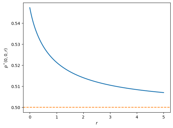
Fig. 104.1 Normalized price against interest rate#
In the first figure, notice that:
The resale option pushes the normalized price \(p^*(0,0,r)\) above fundamentals \((0.5)\) for any finite \(r\).
As \(r\) increases (\(\beta\) decreases), the option value fades and \(p^*(0,0,r) \to 0.5\).
At \(r = 0.05\) the premium is about \(8–9\%\), consistent with Morris (1996, Section IV).
# Figure II: p*(t/2,t,0.05) as a function of t
r = 0.05
T = 60
p_mat = normalized_price_two_agents(priors[0], priors[1], r, T=T)
t_vals = np.arange(0, 54, 2)
s_vals = t_vals // 2
y = np.array([p_mat[s, t] for s, t in zip(s_vals, t_vals)])

fig, ax = plt.subplots()
ax.plot(t_vals, y, lw=2)
ax.set_xlabel(r'$t$')
ax.set_ylabel(r'$p^*(t/2,t,0.05)$')
ax.axhline(0.5, color='C1', linestyle='--')
plt.show()

p0 = p_mat[0,0]
μ0 = 0.5
print("Initial normalized premium at r=0.05 (%):",
      np.round(100 * (p0 / μ0 - 1.0), 2))
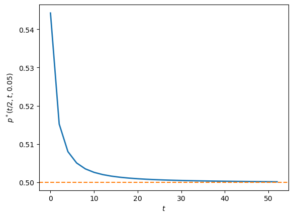
Fig. 104.2 Normalized price against time#
Initial normalized premium at r=0.05 (%): 8.85
In the second figure, notice that:
Along the symmetric path \(s = t/2\), both traders’ fundamental valuations equal \(0.5\) at every \(t\), yet the price starts above \(0.5\) and declines toward \(0.5\) as learning reduces disagreement and the resale option loses value.
104.7.4. General N–trader extension#
The same recursion extends to any finite set of Beta priors \(\{(a_i,b_i)\}_{i=1}^N\) by taking a max over \(i\) each period.
def price_learning(priors, β=0.75, T=200):
    """
    N-trader version with heterogeneous Beta priors.
    """
    price_array = np.zeros((T+1, T+1))

    def perp_i(i, s, t):
        a, b = priors[i]
        return perpetuity_value(a, b, s, t, β)

    # Terminal condition
    for s in range(T+1):
        price_array[s, T] = max(
            perp_i(i, s, T) for i in range(len(priors)))

    # Backward induction
    for t in range(T-1, -1, -1):
        for s in range(t, -1, -1):
            conts = []
            for (a, b) in priors:
                μ = posterior_mean(a, b, s, t)
                conts.append(μ *
                (1.0 + price_array[s+1, t+1])
                     + (1.0 - μ) * price_array[s, t+1])
            price_array[s, t] = β * max(conts)

    return price_array

β = 0.75
priors = [(1,1), (0.5,0.5), (3,2)]
price_N = price_learning(priors, β=β, T=150)

# Compute valuations for each trader at (0,0)
μ_vals = [posterior_mean(a, b, 0, 0) for a, b in priors]
perp_vals = [(β / (1 - β)) * μ for μ in μ_vals]

print("Three-trader example at (s,t)=(0,0):")
print(f"Price at (0,0) = {np.round(price_N[0,0], 6)}")
print(f"\nTrader valuations:")
for i, (μ, perp) in enumerate(zip(μ_vals, perp_vals), 1):
    print(f"  Trader {i} = {np.round(perp, 6)}")
Three-trader example at (s,t)=(0,0):
Price at (0,0) = 1.937972

Trader valuations:
  Trader 1 = 1.5
  Trader 2 = 1.5
  Trader 3 = 1.8
Note that the asset price is above all traders’ valuations.
Morris tells us that no rate dominance exists in this case.
Let’s verify this using the code below
dominant = None
for i in range(len(priors)):
    is_dom = all(
        priors[i][0] >= priors[j][0] and priors[i][1] <= priors[j][1]
                 for j in range(len(priors)) if i != j)
    if is_dom:
        dominant = i
        break

if dominant is not None:
    print(f"\nTrader {dominant+1} is the global optimist (rate-dominant)")
else:
    print(f"\nNo global optimist and speculative premium exists")
No global optimist and speculative premium exists
Indeed, there is no global optimist and a speculative premium exists.
104.8. Concluding remarks#
Morris [1996] uses his model to interpret a ‘‘hot issue’’ anomaly described by [Miller, 1977] according to which opening market prices of initial public offerings seem higher than values prices that emerge later.
104.9. Exercise#
Exercise 104.1
Morris [Morris, 1996] provides a sharp characterization of when speculative bubbles arise.
The key condition is that there is no global optimist.
In this exercise, you will verify this condition for the following sets of traders with Beta priors:
Trader 1: \(\text{Beta}(2,1)\), Trader 2: \(\text{Beta}(1,2)\)
Trader 1: \(\text{Beta}(1,1)\), Trader 2: \(\text{Beta}(1/2,1/2)\)
Trader 1: \(\text{Beta}(3,1)\), Trader 2: \(\text{Beta}(2,1)\), Trader 3: \(\text{Beta}(1,2)\)
Trader 1: \(\text{Beta}(1,1)\), Trader 2: \(\text{Beta}(1/2,1/2)\), Trader 3: \(\text{Beta}(3/2,3/2)\)
Solution
Here is one solution:
def check_rate_dominance(priors):
    """
    Check if any trader rate-dominates all others.
    """
    N = len(priors)

    for i in range(N):
        a_i, b_i = priors[i]
        is_dominant = True

        for j in range(N):
            if i == j:
                continue
            a_j, b_j = priors[j]

            # Check rate dominance condition
            if not (a_i >= a_j and b_i <= b_j):
                is_dominant = False
                break

        if is_dominant:
            return i

    return None

# Test cases
test_cases = [
    ([(2, 1), (1, 2)], "Global optimist exists"),
    ([(1, 1), (0.5, 0.5)], "Perpetual switching"),
    ([(3, 1), (2, 1), (1, 2)], "Three traders with dominant"),
    ([(1, 1), (0.5, 0.5), (1.5, 1.5)], "Three traders, no dominant")
]

for priors, description in test_cases:
    dominant = check_rate_dominance(priors)

    print(f"\n{description}")
    print(f"Priors: {priors}")
    print("=="*8)
    if dominant is not None:
        print(f"Trader {dominant+1} is the global optimist (rate-dominant)")
    else:
        print(f"No global optimist exists")
    print("=="*8 + "\n")
Global optimist exists
Priors: [(2, 1), (1, 2)]
================
Trader 1 is the global optimist (rate-dominant)
================


Perpetual switching
Priors: [(1, 1), (0.5, 0.5)]
================
No global optimist exists
================


Three traders with dominant
Priors: [(3, 1), (2, 1), (1, 2)]
================
Trader 1 is the global optimist (rate-dominant)
================


Three traders, no dominant
Priors: [(1, 1), (0.5, 0.5), (1.5, 1.5)]
================
No global optimist exists
================