108. Drifts and Volatilities after 2000#
108.1. Overview#
Drifts and Volatilities fit the Bayesian vector autoregression of Cogley and Sargent [2005], with drifting coefficients and stochastic volatilities, to quarterly U.S. data on interest, unemployment, and inflation for 1959–2000.
It found that both the volatilities and the coefficients drifted: shocks were large around 1980, and core inflation and inflation persistence rose through the 1970s and fell together after 1980.
Cogley and Sargent’s sample ends in 2000, so it misses the financial crisis, the long stretch at the zero lower bound, the pandemic, and the 2021–2022 inflation surge.
This lecture re-estimates the same model, with the same priors and the same 1948–1958 training sample, on data extended through the latest complete quarter, and asks two questions.
Do the new observations change what the model says about 1959–2000?
Did the recent inflation surge bring back 1970s-style persistence?
The code repeats that of Drifts and Volatilities, where each piece is explained; it is collapsed below so that this lecture runs on its own.
We begin with imports and the addresses of the data.
import time

import matplotlib.pyplot as plt
import numpy as np
import pandas as pd
from scipy import linalg
from scipy.special import expit
from threadpoolctl import threadpool_limits

# The matrices in this lecture are small, so extra BLAS threads only add overhead.
threadpool_limits(1)

archive_url = 'https://github.com/QuantEcon/data-lectures/raw/main/lectures/NEWQDATA.csv'
fred_url = ('https://fred.stlouisfed.org/graph/fredgraph.csv?'
            'id=CPIAUCSL%2CUNRATE%2CTB3MS')
108.2. The model and the sampler#
The model is the one in A VAR with drifting coefficients and stochastic volatility: a VAR(2) in the nominal interest rate, the logit of unemployment, and inflation, \(y_t = X_t^\top\theta_t+\varepsilon_t\), whose coefficients follow a random walk \(\theta_t=\theta_{t-1}+v_t\) with \(v_t\sim N(0,Q)\), restricted to stable paths, and whose innovation covariance \(R_t=B^{-1}H_tB^{-1\prime}\) has random-walk log volatilities.
The first cell builds the model, the data, and the priors.
The second cell is the sampler of Simulating the posterior: a Carter–Kohn draw of the coefficient path, redrawn until it is stable, followed by the updates of \(Q\), the volatility scales \(\sigma\), the covariance parameters \(\beta\), and the volatility paths.
The third cell computes the summaries of What the data say: the posterior mean of \(R_t\), core inflation and the natural rate, and the normalized inflation spectrum \(g_{\pi\pi}(\omega,t)\).
108.3. The extended sample#
We keep Cogley and Sargent’s archived data through 2000Q4 and append newer observations from FRED: seasonally adjusted CPI, seasonally adjusted unemployment, and the three-month Treasury-bill rate.
The transformations and within-quarter timing are unchanged: CPI comes from the third month of each quarter, unemployment is a three-month average, and the interest rate comes from the first month.
Keeping the archive for 1948–2000 means that revisions to old data are not mistaken for information in the new quarters; the first appended inflation rate uses revised CPI levels for both 2000Q4 and 2001Q1.
As the BLS notes, the October 2025 unemployment rate was never collected, because of the federal government shutdown, so 2025Q4 lacks one of its three months.
Rather than end the sample at 2025Q3 forever, we fill isolated missing months by linear interpolation between their neighbors, and we print the months filled.
The sample then ends at the last quarter for which all three series are complete, found automatically.
archive = pd.read_csv(archive_url)
fred = pd.read_csv(fred_url, parse_dates=['observation_date'],
                   index_col='observation_date')

unrate = fred['UNRATE'].dropna()
unrate = unrate.reindex(pd.date_range(unrate.index[0], unrate.index[-1],
                                      freq='MS'))
filled_months = list(unrate.index[unrate.isna()].strftime('%Y-%m'))
unrate = unrate.interpolate(limit=1, limit_area='inside')


def by_quarter(series, months):
    """Observations from the given months of each quarter, indexed by quarter."""
    picked = series[series.index.month.isin(months)].dropna()
    picked.index = picked.index.to_period('Q')
    return picked


month_counts = unrate.groupby(unrate.index.to_period('Q')).count()
table = pd.concat({
    'interest': by_quarter(fred['TB3MS'], (1, 4, 7, 10)),
    'cpi': by_quarter(fred['CPIAUCSL'], (3, 6, 9, 12)),
    'unemployment': unrate.groupby(unrate.index.to_period('Q')).mean()[
        month_counts == 3],
}, axis=1)
table['y3'] = table['interest'] / (400 - table['interest'])
table['ur'] = table['unemployment'] / 100
table['dp'] = np.log(table['cpi']).diff()
table['date'] = table.index.year + (table.index.quarter - 1) / 4

extension = table.loc['2001Q1':, ['date', 'y3', 'ur', 'dp']]
incomplete = extension.index[extension.isna().any(axis=1)]
if len(incomplete):
    extension = extension.loc[:incomplete[0] - 1]
spliced = pd.concat((archive, extension.reset_index(drop=True)),
                    ignore_index=True)
assert np.allclose(np.diff(spliced['date']), 0.25)
sample_end = extension.index[-1]

print('months filled by interpolation:', filled_months)
print('last quarter of the sample:', sample_end)
months filled by interpolation: ['2025-10']
last quarter of the sample: 2026Q3
The next figure shows the data, with a dashed line at the end of Cogley and Sargent’s sample.
shown = spliced[spliced['date'] >= 1959]
fig, axes = plt.subplots(3, 1, figsize=(9, 7), sharex=True)
axes[0].plot(shown['date'], 400 * shown['dp'], lw=2)
axes[0].set_ylabel('inflation (annual %)')
axes[1].plot(shown['date'], 100 * shown['ur'], lw=2)
axes[1].set_ylabel('unemployment (%)')
axes[2].plot(shown['date'], 400 * shown['y3'] / (1 + shown['y3']), lw=2)
axes[2].set_ylabel('interest (annual %)')
axes[2].set_xlabel('year')
for ax in axes:
    ax.axvline(2000.75, color='0.6', ls='--', lw=1)
plt.tight_layout()
plt.show()
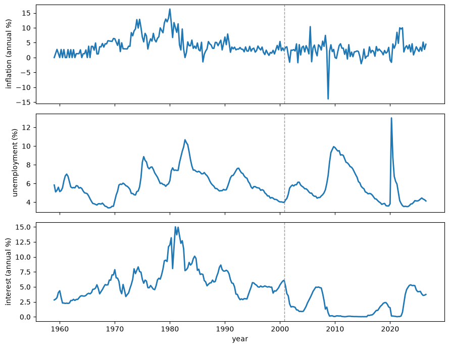
Fig. 108.1 Observed \(\pi_t\), \(u_t\), and \(i_t\) in the extended sample#
The extension adds the financial-crisis recession, a pandemic spike in quarterly unemployment, a short inflation surge in 2021–2022, and two long stretches of near-zero interest rates.
Because inflation is annualized from quarterly changes, isolated movements look large, but the recent surge is much shorter than the sustained rise of the 1970s.
108.4. Fitting the extended sample#
The sample is now much longer, and stable coefficient paths are much harder to draw over it, so a sweep costs several times more than in Drifts and Volatilities.
To bound the cost, a sweep tries at most 50 backward passes before keeping the current path, which still leaves the posterior invariant (the table reports how often that happens), and we run 10,000 sweeps, discard the first 1,000, and keep every 5th of the rest.
data = prepare_data(spliced)
prior = calibrate_prior(data)
burn = 1_000
posterior = run_sampler(data['y'], data['x'], prior,
                        n_sweeps=10_000, burn=burn, thin=5, seed=42)

dates = data['dates']
years = np.floor(dates + 1e-8).astype(int)
annual = np.array([np.flatnonzero(years == year)[-1]
                   for year in np.unique(years)])
trace_q = posterior['trace_q'][burn:]
τ = integrated_autocorrelation_time(trace_q)
passes = posterior['passes'][burn:]

pd.Series({
    'run time (minutes)': posterior['minutes'],
    'quarters in the estimation sample': len(dates),
    'retained draws': len(posterior['β']),
    'mean backward passes per sweep': passes.mean(),
    'sweeps that kept the current path': np.sum(passes > 50),
    'autocorrelation time of tr(Q)': τ,
    'effective sample size of tr(Q)': len(trace_q) / τ,
}, name='value').to_frame().round(3)
| value | |
|---|---|
| run time (minutes) | 12.484 |
| quarters in the estimation sample | 271.000 |
| retained draws | 1800.000 |
| mean backward passes per sweep | 18.675 |
| sweeps that kept the current path | 1834.000 |
| autocorrelation time of tr(Q) | 992.580 |
| effective sample size of tr(Q) | 9.067 |
As in Drifts and Volatilities, the chain moves slowly in the direction of \(Q\), and with fewer sweeps the effective sample size of \(\operatorname{tr}(Q)\) is even smaller, so magnitudes that depend on \(Q\) carry large Monte Carlo error; the text relies only on features that held in runs with other seeds.
108.5. Did coefficient drift continue?#
The histogram shows \(\operatorname{tr}(Q)\) at every sweep after the burn-in.
fig, ax = plt.subplots()
ax.hist(trace_q, bins=50, histtype='step', lw=2)
ax.axvline(np.trace(prior['q_center']), color='C1', lw=2,
           label=r'prior $\mathrm{tr}(\bar Q)$')
ax.set_xlabel(r'$\mathrm{tr}(Q)$')
ax.set_ylabel('sweeps')
ax.legend()
plt.show()
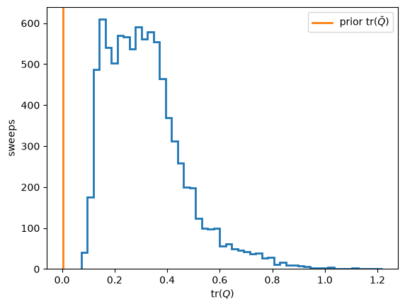
Fig. 108.2 Posterior \(\operatorname{tr}(Q)\) in the extended sample and prior \(\operatorname{tr}(\bar Q)\)#
The table below gives the numbers behind the figure.
q_eigenvalues = np.linalg.eigvalsh(posterior['Q'].mean(axis=0))[::-1]
pd.Series({
    'posterior mean of tr(Q)': trace_q.mean(),
    'smallest tr(Q) / tr(Q bar)': trace_q.min() / np.trace(prior['q_center']),
    'share of the first principal component': q_eigenvalues[0] / q_eigenvalues.sum(),
    'share of the first three': q_eigenvalues[:3].sum() / q_eigenvalues.sum(),
}, name='value').to_frame().round(3)
| value | |
|---|---|
| posterior mean of tr(Q) | 0.318 |
| smallest tr(Q) / tr(Q bar) | 24.456 |
| share of the first principal component | 0.639 |
| share of the first three | 0.976 |
The drift rate is several times larger than in the 1959–2000 fit of Drifts and Volatilities, and the drift is concentrated in even fewer directions.
The chain explores this posterior very slowly: in runs with other seeds the posterior mean of \(\operatorname{tr}(Q)\) differed by a factor of more than two, although it was always several times the 1959–2000 value.
One likely contributor is the pandemic: in 2020Q2 the logit of unemployment jumped by dozens of innovation standard deviations, far more than a random-walk volatility can absorb within a quarter, so part of the jump is attributed to the coefficients.
Because \(Q\) is a single drift covariance for the whole sample, this histogram cannot by itself say whether drift slowed or sped up after 2000; for that we look at what the coefficients imply.
108.6. Volatility after the Great Moderation#
The innovation standard deviations and correlations come from the posterior mean \(\mathbb{E}(R_t\mid T)\), as in Drifts and Volatilities.
r_mean = mean_innovation_covariance(posterior['h'], posterior['β'])
sd = 1e4 * np.sqrt(np.diagonal(r_mean, axis1=1, axis2=2))


def correlation(left, right):
    return r_mean[:, left, right] / np.sqrt(r_mean[:, left, left]
                                            * r_mean[:, right, right])


fig, axes = plt.subplots(3, 2, figsize=(9, 8), sharex=True)
for row, (index, label) in enumerate(((0, 'Nominal interest'),
                                      (2, 'Inflation'), (1, 'Unemployment'))):
    axes[row, 0].plot(dates, sd[:, index], lw=2)
    axes[row, 0].set_title(label)
for row, (left, right, label) in enumerate(((0, 1, 'Interest--unemployment'),
                                            (0, 2, 'Interest--inflation'),
                                            (2, 1, 'Inflation--unemployment'))):
    axes[row, 1].plot(dates, correlation(left, right), lw=2)
    axes[row, 1].set_title(label)
for ax in axes.flat:
    ax.axvline(2000.75, color='0.6', ls='--', lw=1)
axes[1, 0].set_ylabel(r'standard deviation $\times 10^4$')
axes[1, 1].set_ylabel('correlation')
axes[-1, 0].set_xlabel('year')
axes[-1, 1].set_xlabel('year')
plt.tight_layout()
plt.show()
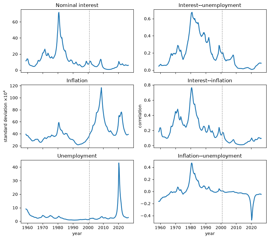
Fig. 108.3 Standard deviations and correlations implied by \(E(R_t\mid T)\), extended sample#
The table below gives the numbers behind the figure.
pd.DataFrame({
    'peak date': [dates[np.argmax(sd[:, i])] for i in range(3)],
    'standard deviation at the end': sd[-1],
}, index=['interest', 'unemployment', 'inflation']).round(2)
| peak date | standard deviation at the end | |
|---|---|---|
| interest | 1980.75 | 6.02 |
| unemployment | 2020.25 | 2.77 |
| inflation | 2008.75 | 38.97 |
The Volcker years still dominate interest-rate innovations, the financial crisis produces the largest inflation innovations, and the pandemic produces by far the largest unemployment innovations, together with a sharp swing in the inflation–unemployment correlation.
Recent episodes thus changed the size and composition of reduced-form shocks dramatically, which is direct evidence for a bad-luck component, although reduced-form innovations are not structural shocks.
The generalized innovation variance \(\log|\mathbb{E}(R_t\mid T)|\) summarizes the total one-step uncertainty.
logdet_r = np.linalg.slogdet(r_mean)[1]
fig, ax = plt.subplots()
ax.plot(dates, logdet_r, lw=2)
ax.axvline(2000.75, color='0.6', ls='--', lw=1)
ax.set_xlabel('year')
ax.set_ylabel(r'$\log |E(R_t\mid T)|$')
plt.show()
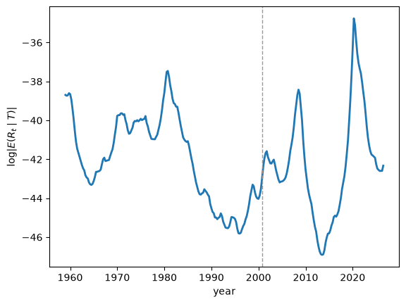
Fig. 108.4 Generalized innovation variance \(\log |E(R_t\mid T)|\), extended sample#
The table below gives the numbers behind the figure.
def period_mean(values, first, last):
    """Average a quarterly series over the years first, ..., last."""
    return values[(years >= first) & (years <= last)].mean()


display_periods = {'1980--1982': (1980, 1982), '1990--2000': (1990, 2000),
                   '2010--2015': (2010, 2015), '2020--2021': (2020, 2021)}


def extreme(values, first, last, statistic):
    return statistic(values[(years >= first) & (years <= last)])


pd.DataFrame({
    'interest innovation sd (basis points)': [
        period_mean(sd[:, 0], *p) for p in display_periods.values()],
    'interest-inflation correlation': [
        period_mean(correlation(0, 2), *p) for p in display_periods.values()],
    'log |E(R_t | T)|, max or min': [
        extreme(logdet_r, 1980, 1982, np.max), extreme(logdet_r, 1990, 2000, np.min),
        extreme(logdet_r, 2010, 2015, np.min), extreme(logdet_r, 2020, 2021, np.max)],
}, index=display_periods.keys()).round(3)
| interest innovation sd (basis points) | interest-inflation correlation | log |E(R_t | T)|, max or min | |
|---|---|---|---|
| 1980--1982 | 52.647 | 0.645 | -37.459 |
| 1990--2000 | 7.133 | 0.172 | -45.819 |
| 2010--2015 | 1.333 | 0.015 | -46.911 |
| 2020--2021 | 8.145 | 0.075 | -34.759 |
Joint innovation variance rises in the financial crisis, falls to a trough in the early 2010s deeper than its 1990s low, and jumps in 2020 above even its 1981 peak before falling back.
The trough is not a second Great Moderation.
At the zero lower bound the Treasury-bill rate barely moved, so its innovations nearly vanished and lost their correlation with inflation innovations, as the table shows, and the log determinant collapses with them.
For the same reason a short-rate measure of policy activism carries little information after 2008, and we do not compute one here.
108.7. Core inflation, the natural rate, and persistence#
We compute core inflation, the natural rate, and \(g_{\pi\pi}(0,t)\) from every retained draw, as in Inflation persistence.
feature_draws = posterior_feature_draws(posterior, annual)
medians = {key: np.median(value, axis=1) for key, value in feature_draws.items()}

fig, axes = plt.subplots(3, 1, figsize=(9, 8), sharex=True)
for ax, (key, ylabel) in zip(axes, (('core', 'core inflation (%)'),
                                    ('natural', 'natural rate (%)'),
                                    ('persistence', r'$g_{\pi\pi}(0,t)$'))):
    lower, upper = np.quantile(feature_draws[key], (0.05, 0.95), axis=1)
    line, = ax.plot(dates[annual], medians[key], lw=2)
    ax.fill_between(dates[annual], lower, upper, color=line.get_color(),
                    alpha=0.2)
    ax.axvline(2000.75, color='0.6', ls='--', lw=1)
    ax.set_ylabel(ylabel)
axes[2].axhline(1 / (2 * np.pi), color='0.45', ls=':', lw=1)
axes[-1].set_xlabel('year')
plt.tight_layout()
plt.show()
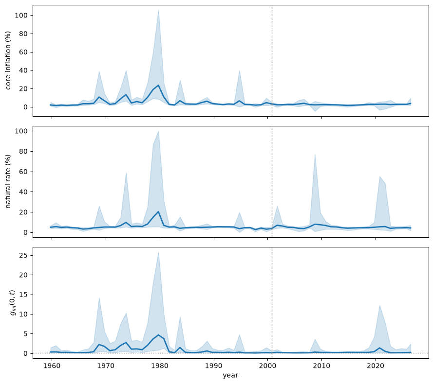
Fig. 108.5 Posterior medians and pointwise 90 percent intervals for \(\bar\pi_t\), \(\bar u_t\), and \(g_{\pi\pi}(0,t)\), extended sample#
The dotted line in the bottom panel is the white-noise value \(1/(2\pi)\).
The table summarizes the posterior medians by period.
annual_years = years[annual]


def median_summary(key, first, last, statistic=np.mean):
    """Apply a statistic to the annual posterior medians over first, ..., last."""
    mask = (annual_years >= first) & (annual_years <= last)
    return statistic(medians[key][mask])


core_peak = np.argmax(medians['core'] * (annual_years <= 2000))
pd.Series({
    'core inflation, 1970s peak (%)': medians['core'][core_peak],
    'year of the core peak': annual_years[core_peak],
    'natural rate, 1970--1979 range (%)': (
        f"{median_summary('natural', 1970, 1979, np.min):.1f}--"
        f"{median_summary('natural', 1970, 1979, np.max):.1f}"),
    'g(0), 1970--1979 mean': median_summary('persistence', 1970, 1979),
    'last year before 2001 with g(0) > 1': annual_years[
        (annual_years <= 2000) & (medians['persistence'] > 1)].max(),
    'core inflation, 2001--2019 range (%)': (
        f"{median_summary('core', 2001, 2019, np.min):.1f}--"
        f"{median_summary('core', 2001, 2019, np.max):.1f}"),
    'core inflation, 2020 onward mean (%)': median_summary('core', 2020, 2100),
    'g(0), 2001--2019 mean': median_summary('persistence', 2001, 2019),
    'g(0), 2020 onward mean': median_summary('persistence', 2020, 2100),
}, name='posterior median').to_frame()
| posterior median | |
|---|---|
| core inflation, 1970s peak (%) | 23.596626 |
| year of the core peak | 1979 |
| natural rate, 1970--1979 range (%) | 5.1--20.4 |
| g(0), 1970--1979 mean | 1.973974 |
| last year before 2001 with g(0) > 1 | 1983 |
| core inflation, 2001--2019 range (%) | 1.5--3.8 |
| core inflation, 2020 onward mean (%) | 2.859929 |
| g(0), 2001--2019 mean | 0.201675 |
| g(0), 2020 onward mean | 0.385413 |
Adding a quarter-century of data changes the estimated history of 1959–2000 a great deal.
With the larger drift rate, many draws put a root of the late-1970s VAR close to the unit circle, so the medians of core inflation and of the natural rate around 1979 are higher than in Drifts and Volatilities, in some runs far higher, their bands are enormous, and persistence stays above one until 1980 or later.
How large these numbers are depends on how far the chain has wandered into the tail of \(Q\), and they differed a lot across runs with other seeds; what survives in all runs is the shape: core inflation and persistence rise through the 1970s and collapse in the early 1980s.
After 2000 the picture is calm and robust.
Core inflation stays below about 4 percent, and persistence stays close to the white-noise value, apart from a brief rise around 2020–2021 that is far smaller than in the 1970s and soon reverses.
A burst of large inflation innovations kept measured inflation high for several quarters in 2021–2022 without the strong propagation that the model finds in the 1970s.
The normalized spectrum over all frequencies shows the same thing.
θ_mean = posterior['θ'].mean(axis=0)
frequencies = np.linspace(0, 0.5, 41)
normalized = np.column_stack([
    inflation_spectrum(θ_mean[:, t], r_mean[t], frequencies)[1]
    for t in range(len(dates))
])
fig, ax = plt.subplots(figsize=(8, 4))
image = ax.pcolormesh(dates, frequencies, np.log10(normalized), shading='auto')
ax.axvline(2000.75, color='0.9', ls='--', lw=1)
ax.set_xlabel('year')
ax.set_ylabel('cycles per quarter')
fig.colorbar(image, ax=ax, label=r'$\log_{10} g_{\pi\pi}(\omega,t)$')
plt.show()
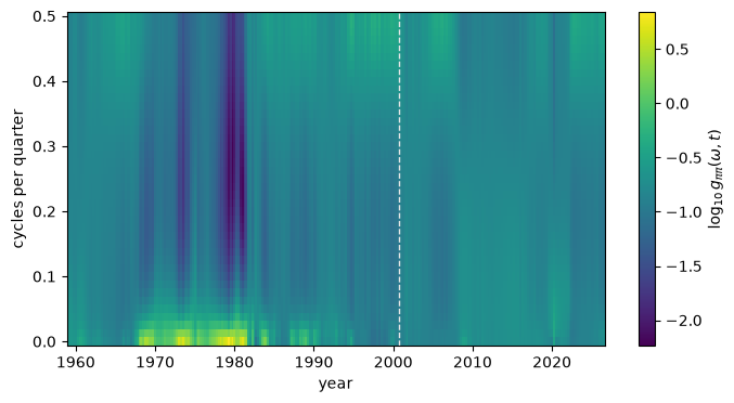
Fig. 108.6 Normalized inflation spectrum \(g_{\pi\pi}(\omega,t)\), extended sample#
The normalized spectrum has a low-frequency ridge from the late 1960s to the early 1980s and, after 2000, only a brief one around 2020: the recent inflation surge shows up mainly as large shocks, not as lasting stronger propagation.
108.7.1. Two measures of persistence#
The Lost Conquest: Fed Policy in the 2020s gives the Fed a learning model in which perceived persistence is the coefficient on lagged inflation in a regression of year-over-year inflation on its own lag, sampled quarterly.
Year-over-year rates overlap: consecutive values share three of their four quarters.
Even if quarterly inflation were white noise, year-over-year inflation sampled quarterly would have a first-order autocorrelation of \(3/4\), so a persistence measure based on it is pushed toward one and falls later and less than a measure based on quarterly rates.
The next cell compares least-squares \(AR(1)\) coefficients of the two inflation rates in our data, period by period; Exercise 109.5 reruns that lecture’s learning Fed on quarterly inflation.
cpi_inflation = pd.Series(400 * spliced['dp'].to_numpy(), index=spliced['date'])
year_over_year = cpi_inflation.rolling(4).mean()


def ar1_coefficient(series, first, last):
    """Least-squares AR(1) slope over the years first, ..., last."""
    z = series[(series.index >= first) & (series.index < last + 1)].dropna()
    X = np.column_stack((np.ones(len(z) - 1), z.to_numpy()[:-1]))
    return np.linalg.lstsq(X, z.to_numpy()[1:], rcond=None)[0][1]


periods = ((1960, 1969), (1970, 1979), (1985, 1999), (2000, 2019), (2020, 2100))
pd.DataFrame({
    'quarterly inflation': [ar1_coefficient(cpi_inflation, *p) for p in periods],
    'year-over-year inflation': [ar1_coefficient(year_over_year, *p)
                                 for p in periods],
}, index=['1960s', '1970s', '1985--1999', '2000--2019', '2020 onward']).round(2)
| quarterly inflation | year-over-year inflation | |
|---|---|---|
| 1960s | 0.43 | 1.02 |
| 1970s | 0.80 | 1.01 |
| 1985--1999 | 0.37 | 0.89 |
| 2000--2019 | -0.05 | 0.68 |
| 2020 onward | 0.43 | 0.87 |
The \(AR(1)\) coefficient of year-over-year inflation is near one in the 1960s and 1970s, and it stays high after 1985 and even in 2000–2019, when the coefficient for quarterly inflation is about zero.
The overlap both inflates the year-over-year measure and blunts its decline, which is why the perceived persistence in The Lost Conquest: Fed Policy in the 2020s falls later and less than the quarterly measures here and in Drifts and Volatilities.
108.8. What the additional observations change#
The extra quarter-century strengthens the bad-luck evidence for the recent period.
It adds large volatility episodes, the financial crisis in inflation and the pandemic in unemployment, and a zero-lower-bound period in which the short rate says little about policy.
The recent inflation surge did not bring back 1970s-style propagation: persistence after 2000 stays near the white-noise value, and core inflation stays low.
The drift rate, and with it the estimated history of the 1970s, becomes much harder to pin down: the posterior puts weight on far faster drift than the 1959–2000 fit, and a chain short enough for a lecture cannot explore that tail reliably, so magnitudes that depend on \(Q\) should not be taken at face value.
The shape of the earlier drift documented in Drifts and Volatilities survives: persistence and core inflation still rise in the 1970s and fall in the early 1980s.
The next and last lecture, The Lost Conquest: Fed Policy in the 2020s, returns to a learning Fed: it asks whether drifting beliefs about persistence and the slope of the Phillips curve, of the kind that Adaptive Learning and Escape Dynamics and Priors, Escapes, and Learning Cycles model, help explain the Fed’s slow response to the inflation of 2021–2022, and so whether the conquest of American inflation was lost.
108.9. Exercises#
Exercise 108.1
Sims [2001] pointed out that filtered estimates of drifting coefficients wander even when the true coefficients are constant, which is why Cogley and Sargent [2005] report smoothed estimates.
Simulate \(y_t=\rho_t y_{t-1}+w_t\), \(w_t\sim N(0,1)\), for \(T=168\) quarters in two cases: (a) \(\rho_t=0.5\) for all \(t\), and (b) \(\rho_t\) a random walk that starts at \(0.5\) with innovation variance \(4\times 10^{-4}\).
In each case run the scalar Kalman filter of A First Look at the Kalman Filter that treats \(\rho_t\) as a random walk with innovation variance \(q=4\times 10^{-4}\), starting from mean 0 and variance 1, and then the smoother of Appendix: the sampler in detail.
Compare the standard deviations over time of the true, filtered, and smoothed paths, ignoring the first 20 quarters.
What does the smoothed path look like if the filter assumes \(q=0\)?
At the last date of a sample the smoothed and filtered estimates coincide.
What does that imply for the estimates in this lecture that bear on the 2020s?
Solution
Here is one solution.
def tvp_ar1(T, ρ0, q, rng):
    """Simulate y_t = ρ_t y_{t-1} + w_t with ρ_t a random walk."""
    ρ = ρ0 + np.r_[0, np.cumsum(np.sqrt(q) * rng.standard_normal(T))]
    y = np.zeros(T + 1)
    for t in range(1, T + 1):
        y[t] = ρ[t] * y[t - 1] + rng.standard_normal()
    return y, ρ


def filter_and_smooth(y, q, mean0=0.0, var0=1.0):
    """Scalar Kalman filter and Rauch-Tung-Striebel smoother for ρ_t."""
    T = len(y) - 1
    m, P, P_pred = np.empty(T + 1), np.empty(T + 1), np.empty(T + 1)
    m[0], P[0] = mean0, var0
    for t in range(1, T + 1):
        P_pred[t] = P[t - 1] + q
        K = P_pred[t] * y[t - 1] / (y[t - 1]**2 * P_pred[t] + 1)
        m[t] = m[t - 1] + K * (y[t] - y[t - 1] * m[t - 1])
        P[t] = P_pred[t] - K * y[t - 1] * P_pred[t]
    s = m.copy()
    for t in range(T - 1, -1, -1):
        s[t] = m[t] + P[t] / P_pred[t + 1] * (s[t + 1] - m[t])
    return m, s


rng = np.random.default_rng(3)
fig, axes = plt.subplots(1, 2, figsize=(10, 3.8), sharey=True)
rows = {}
for ax, (q_true, title) in zip(axes, ((0.0, r'constant $\rho$'),
                                      (4e-4, r'drifting $\rho$'))):
    y, ρ = tvp_ar1(168, 0.5, q_true, rng)
    filtered, smoothed = filter_and_smooth(y, q=4e-4)
    _, flat = filter_and_smooth(y, q=0.0)
    for path, label in ((ρ, 'true'), (filtered, 'filtered'),
                        (smoothed, 'smoothed')):
        ax.plot(path[1:], lw=2 if label == 'true' else 1.5, label=label)
    ax.set_title(title)
    ax.set_xlabel('quarter')
    rows[title] = {'true': ρ[20:].std(), 'filtered': filtered[20:].std(),
                   'smoothed': smoothed[20:].std(),
                   'smoothed, q = 0': flat[20:].std()}
axes[0].set_ylabel(r'$\rho_t$')
axes[0].legend()
plt.tight_layout()
plt.show()
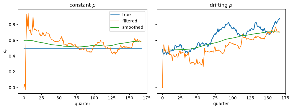
The table below gives the numbers behind the figure.
pd.DataFrame(rows).T.round(3)
| true | filtered | smoothed | smoothed, q = 0 | |
|---|---|---|---|---|
| constant $\rho$ | 0.000 | 0.070 | 0.022 | 0.0 |
| drifting $\rho$ | 0.117 | 0.127 | 0.081 | 0.0 |
When \(\rho\) is constant, the filtered estimate wanders, with a standard deviation over time several times that of the smoothed estimate, which is nearly flat; that is Sims’s point.
When \(\rho\) drifts, the filtered path adds transient noise to the drift, while the smoothed path is smoother than the truth.
With \(q=0\) the smoother returns an exactly flat path, as in Cogley and Sargent’s footnote 16: the backward pass has \(J_t=1\) and no noise, so every date receives the end-of-sample estimate.
Near the end of a sample the smoother has few later observations to draw on, so its estimates behave more like filtered ones, and at the last date they are the filtered estimate.
The estimates for the 2020s in this lecture therefore carry some of the transient wandering that Sims warned about, and they will be revised as new quarters arrive, which is one more reason to read the endpoint bands in Core inflation, the natural rate, and persistence with care.
Exercise 108.2
A Kalman filter on coefficients that drift as random walks behaves like constant-gain least squares, and this exercise asks how large the implied gain is.
For the local-level model \(y_t=\mu_t+w_t\), \(\mu_t=\mu_{t-1}+v_t\), with \(\mathbb{V}[w_t]=1\) and \(\mathbb{V}[v_t]=q\), show that the steady-state predicted variance is \(p=(q+\sqrt{q^2+4q})/2\) and the steady-state Kalman gain is \(K=p/(1+p)\approx\sqrt q\) for small \(q\). Check this numerically by iterating the Riccati equation for \(q\in\{10^{-4},10^{-3},10^{-2}\}\).
Run the Kalman filter of Appendix: the sampler in detail for the 21 coefficients with \(Q\) and \(R_t\) fixed at their posterior means. At each date compute \(w_t\), the weight that the updated fitted value of inflation puts on the newest inflation forecast error, which is the \((3,3)\) element of \(X_t^\top K_t\).
Under constant-gain least squares, that weight is the gain times \(x_t^\top R^{-1}x_t\), where \(R\) is the regressors’ second-moment matrix, and \(x_t^\top R^{-1}x_t\) averages \(k\), the number of regressors. Convert \(w_t\) into an equivalent gain \(w_t/7\) and compare its average by decade with the gains used in this section: 0.025 in Adaptive Learning and Escape Dynamics, 0.02 in A government learning the Phillips curve, and 0.03 in The Lost Conquest: Fed Policy in the 2020s.
Solution
In steady state the predicted variance satisfies \(p = p - p^2/(p+1) + q\), so \(p^2 - qp - q = 0\) and \(p=(q+\sqrt{q^2+4q})/2\approx\sqrt q\), which gives \(K=p/(1+p)\approx\sqrt q\).
for q in (1e-4, 1e-3, 1e-2):
    p = 1.0
    for _ in range(10_000):
        p = p - p**2 / (p + 1) + q
    formula = (q + np.sqrt(q**2 + 4 * q)) / 2
    print(f'q = {q:g}: iterated gain {p / (1 + p):.4f}, '
          f'formula {formula / (1 + formula):.4f}, sqrt(q) {np.sqrt(q):.4f}')
q = 0.0001: iterated gain 0.0100, formula 0.0100, sqrt(q) 0.0100
q = 0.001: iterated gain 0.0311, formula 0.0311, sqrt(q) 0.0316
q = 0.01: iterated gain 0.0951, formula 0.0951, sqrt(q) 0.1000
For the VAR we run the forward recursion with the posterior means of \(Q\) and \(R_t\) and record the weight on the newest inflation surprise.
q_bar = posterior['Q'].mean(axis=0)
X = design_matrices(data['x'])
P = prior['θ_covariance'].copy()
weight = np.empty(len(dates))
for t in range(len(dates)):
    predicted = P + q_bar
    px = predicted @ X[t].T
    gain = np.linalg.solve(X[t] @ px + r_mean[t], px.T).T
    weight[t] = (X[t] @ gain)[2, 2]
    P = predicted - gain @ px.T

decades = {f'{d}s': (d, d + 9) for d in (1960, 1970, 1980, 1990, 2000, 2010)}
decades['2020 onward'] = (2020, 2100)
pd.DataFrame({
    'weight on newest surprise': [period_mean(weight, *p) for p in decades.values()],
    'equivalent gain per regressor': [period_mean(weight, *p) / 7
                                      for p in decades.values()],
}, index=decades.keys()).round(3)
| weight on newest surprise | equivalent gain per regressor | |
|---|---|---|
| 1960s | 0.383 | 0.055 |
| 1970s | 0.538 | 0.077 |
| 1980s | 0.660 | 0.094 |
| 1990s | 0.477 | 0.068 |
| 2000s | 0.208 | 0.030 |
| 2010s | 0.191 | 0.027 |
| 2020 onward | 0.312 | 0.045 |
The steady-state gain is close to \(\sqrt q\), as the formula says.
For the VAR, the weight on the newest inflation surprise is largest before 2000, when the equivalent gain per regressor is roughly two to five times the 0.025 of Adaptive Learning and Escape Dynamics; after 2000 it falls to between about one and two times that value, close to the gains of 0.02 to 0.03 used in this section.
These gains inherit the uncertainty about \(Q\) noted above, because the gain grows with the drift covariance.
Exercise 108.3
Two Illustrations of the Quantity Theory of Money interprets a long-run slope as a ratio of spectral densities at frequency zero, \(h(0)=S_{yz}(0)/S_z(0)\).
Compute the analogous low-frequency slope of inflation on unemployment implied by the local VAR at each date,
draw by draw, and convert it into percentage points of annual inflation per percentage point of the unemployment rate, using the natural rate \(\bar u_t\) to undo the logit transformation.
Plot the posterior median and a 90 percent band.
When was the low-frequency slope negative, as a long-run Phillips tradeoff would require?
Solution
At frequency zero the companion system gives \(2\pi f(0,t)=(I-A_t)^{-1}\mathcal R_t(I-A_t)^{-\top}\).
Inflation is a quarterly log change, so it is multiplied by 400; the logit satisfies \(du_t = 10^{-4}\,dU/[\bar u_t(1-\bar u_t)]\) when \(dU\) is measured in percentage points.
def low_frequency_slope(θ, covariance):
    """Low-frequency slope of annual inflation on the unemployment rate (pp/pp)."""
    intercept, companion = companion_matrix(θ)
    inverse = np.linalg.inv(np.eye(6) - companion)
    innovation = np.zeros((6, 6))
    innovation[:3, :3] = covariance
    S = inverse @ innovation @ inverse.T
    logit_u = 100 * (inverse @ intercept)[1]
    density = expit(logit_u) * expit(-logit_u)      # u(1 - u) at the natural rate
    if density == 0:                                # natural rate at 0 or 100%
        return np.nan
    return 400 * S[2, 1] / S[1, 1] * 1e-4 / density


slopes = np.array([
    [low_frequency_slope(posterior['θ'][d][:, t],
                         innovation_covariance(posterior['h'][d][t],
                                               posterior['β'][d]))
     for t in annual]
    for d in range(len(posterior['β']))
])
lower, median, upper = np.nanquantile(slopes, (0.05, 0.5, 0.95), axis=0)

fig, ax = plt.subplots()
ax.plot(dates[annual], median, lw=2, label='posterior median')
ax.fill_between(dates[annual], lower, upper, alpha=0.2, label='90 percent band')
ax.axhline(0, color='0.45', lw=1)
ax.axvline(2000.75, color='0.6', ls='--', lw=1)
ax.set_xlabel('year')
ax.set_ylabel(r'$h_{\pi u}(0,t)$, percent per percentage point')
ax.set_ylim(-3, 4)     # a few draws near the unit-root boundary explode
ax.legend()
plt.show()
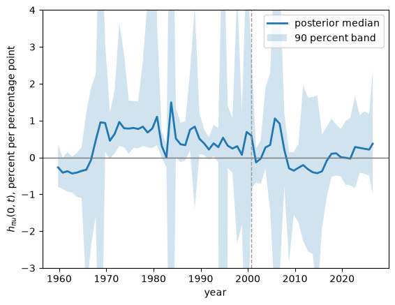
The table below gives the numbers behind the figure.
pd.DataFrame({'5%': lower, 'median': median, '95%': upper},
             index=annual_years).loc[[1962, 1970, 1975, 1980, 1985, 1990, 2000,
                                      2010, 2020, annual_years[-1]]].round(2)
| 5% | median | 95% | |
|---|---|---|---|
| 1962 | -0.95 | -0.44 | 0.02 |
| 1970 | -0.03 | 0.45 | 1.22 |
| 1975 | 0.26 | 0.80 | 1.53 |
| 1980 | 0.33 | 1.10 | 3.62 |
| 1985 | -0.13 | 0.36 | 0.94 |
| 1990 | 0.06 | 0.38 | 0.76 |
| 2000 | -0.86 | 0.59 | 2.85 |
| 2010 | -1.76 | -0.28 | 0.37 |
| 2020 | -0.74 | -0.01 | 0.99 |
| 2026 | -0.97 | 0.37 | 2.36 |
The low-frequency slope is positive in the 1970s, with bands that exclude zero in the second half of the decade: at low frequencies, inflation and unemployment rose together, the opposite of an exploitable long-run tradeoff.
It is negative in the early 1960s, and close to zero and imprecise after 2000.
The vertical axis is cut off because in a few years some draws lie near the unit-root boundary, where the slope explodes.
These are reduced-form statistics: as Sargent [1971] and Lucas [1972] argued, a low-frequency slope is not by itself a structural tradeoff that policy could exploit.