83. A Lake Model of Employment and Unemployment#
GPU
This lecture was built using a machine with access to a GPU — although it will also run without one.
Google Colab has a free tier with GPUs that you can access as follows:
Click on the “play” icon top right
Select Colab
Set the runtime environment to include a GPU
In addition to what’s in Anaconda, this lecture will need the following libraries:
!pip install quantecon jax
83.1. Overview#
This lecture describes what has come to be called a lake model.
The lake model is a basic tool for modeling unemployment.
It allows us to analyze
flows between unemployment and employment
how these flows influence steady state employment and unemployment rates
It is a good model for interpreting monthly labor department reports on gross and net jobs created and destroyed.
The “lakes” in the model are the pools of employed and unemployed.
The “flows” between the lakes are caused by
firing and hiring
entry and exit from the labor force
For the first part of this lecture, the parameters governing transitions into and out of unemployment and employment are exogenous.
Later, we’ll determine some of these transition rates endogenously using the McCall search model.
We’ll also use some nifty concepts like ergodicity, which provides a fundamental link between cross-sectional and long run time series distributions.
These concepts will help us build an equilibrium model of ex-ante homogeneous workers whose different luck generates variations in their ex post experiences.
Let’s start with some imports:
import matplotlib.pyplot as plt
import jax
import jax.numpy as jnp
from typing import NamedTuple
from quantecon.distributions import BetaBinomial
from functools import partial
import jax.scipy.stats as stats
83.1.1. Prerequisites#
Before working through what follows, we recommend you read the lecture on finite Markov chains.
You will also need some basic linear algebra and probability.
83.2. The model#
The economy is inhabited by a very large number of ex-ante identical workers.
The workers live forever, spending their lives moving between unemployment and employment.
Their rates of transition between employment and unemployment are governed by the following parameters:
\(\lambda\), the job finding rate for currently unemployed workers
\(\alpha\), the dismissal rate for currently employed workers
\(b\), the entry rate into the labor force
\(d\), the exit rate from the labor force
The growth rate of the labor force evidently equals \(g=b-d\).
83.2.1. Aggregate variables#
We want to derive the dynamics of the following aggregates:
\(E_t\), the total number of employed workers at date \(t\)
\(U_t\), the total number of unemployed workers at \(t\)
\(N_t\), the number of workers in the labor force at \(t\)
83.2.2. Laws of motion for stock variables#
We begin by constructing laws of motion for the aggregate variables \(E_t,U_t, N_t\).
Of the mass of workers \(E_t\) who are employed at date \(t\),
\((1-d)E_t\) will remain in the labor force
of these, \((1-\alpha)(1-d)E_t\) will remain employed
Of the mass of workers \(U_t\) workers who are currently unemployed,
\((1-d)U_t\) will remain in the labor force
of these, \((1-d) \lambda U_t\) will become employed
Therefore, the number of workers who will be employed at date \(t+1\) will be
A similar analysis implies
The value \(b(E_t+U_t)\) is the mass of new workers entering the labor force unemployed.
The total stock of workers \(N_t=E_t+U_t\) evolves as
Letting \(X_t := \left(\begin{matrix}U_t\\E_t\end{matrix}\right)\), the law of motion for \(X\) is
This law tells us how total employment and unemployment evolve over time.
83.2.3. Laws of motion for rates#
Now let’s derive the law of motion for rates.
We want to track the values of the following objects:
The employment rate \(e_t := E_t/N_t\).
The unemployment rate \(u_t := U_t/N_t\).
(Here and below, capital letters represent aggregates and lowercase letters represent rates)
To get these we can divide both sides of \(X_{t+1} = A X_t\) by \(N_{t+1}\) to get
Letting
we can also write this as
You can check that \(e_t + u_t = 1\) implies that \(e_{t+1}+u_{t+1} = 1\).
This follows from the fact that the columns of \(R\) sum to 1.
83.3. Implementation#
Let’s code up these equations.
83.3.1. Model#
To begin, we set up a class called LakeModel that stores the primitives \(\alpha, \lambda, b, d\).
class LakeModel(NamedTuple):
    """
    Parameters for the lake model
    """
    λ: float
    α: float
    b: float
    d: float
    A: jnp.ndarray
    R: jnp.ndarray
    g: float


def create_lake_model(
        λ: float = 0.283,     # job finding rate
        α: float = 0.013,     # separation rate
        b: float = 0.0124,    # birth rate
        d: float = 0.00822    # death rate
    ) -> LakeModel:
    """
    Create a LakeModel instance with default parameters.

    Computes and stores the transition matrices A and R,
    and the labor force growth rate g.

    """
    # Compute growth rate
    g = b - d

    # Compute transition matrix A
    A = jnp.array([
        [(1-d) * (1-λ) + b, (1-d) * α + b],
        [(1-d) * λ,         (1-d) * (1-α)]
    ])

    # Compute normalized transition matrix R
    R = A / (1 + g)

    return LakeModel(λ=λ, α=α, b=b, d=d, A=A, R=R, g=g)
The default parameter values are:
\(\alpha = 0.013\) and \(\lambda = 0.283\) are based on [Davis et al., 2006]
\(b = 0.0124\) and \(d = 0.00822\) are set to match monthly birth and death rates, respectively, in the U.S. population
As an experiment, let’s create two instances, one with \(α=0.013\) and another with \(α=0.03\)
model = create_lake_model()
print(f"Default α: {model.α}")
print(f"A matrix:\n{model.A}")
print(f"R matrix:\n{model.R}")
Default α: 0.013
A matrix:
[[0.7235063  0.02529314]
 [0.28067374 0.97888684]]
R matrix:
[[0.7204946  0.02518786]
 [0.27950543 0.97481215]]
model_new = create_lake_model(α=0.03)
print(f"New α: {model_new.α}")
print(f"New A matrix:\n{model_new.A}")
print(f"New R matrix:\n{model_new.R}")
New α: 0.03
New A matrix:
[[0.7235063  0.0421534 ]
 [0.28067374 0.9620266 ]]
New R matrix:
[[0.7204946  0.04197793]
 [0.27950543 0.9580221 ]]
83.3.2. Code for dynamics#
We will also use a specialized function to generate time series in an efficient JAX-compatible manner.
Iteratively generating time series is somewhat nontrivial in JAX because arrays are immutable.
Here we use lax.scan, which allows the function to be jit-compiled.
Readers who prefer to skip the details can safely continue reading after the function definition.
@partial(jax.jit, static_argnames=['f', 'num_steps'])
def generate_path(f, initial_state, num_steps, **kwargs):
    """
    Generate a time series by repeatedly applying an update rule.

    Given a map f, initial state x_0, and model parameters, this
    function computes and returns the sequence {x_t}_{t=0}^{T-1} when

        x_{t+1} = f(x_t, **kwargs)

    Args:
        f: Update function mapping (x_t, **kwargs) -> x_{t+1}
        initial_state: Initial state x_0
        num_steps: Number of time steps T to simulate
        **kwargs: Optional extra arguments passed to f

    Returns:
        Array of shape (dim(x), T) containing the time series path
        [x_0, x_1, x_2, ..., x_{T-1}]
    """

    def update_wrapper(state, t):
        """
        Wrapper function that adapts f for use with JAX scan.
        """
        next_state = f(state, **kwargs)
        return next_state, state

    _, path = jax.lax.scan(update_wrapper,
                    initial_state, jnp.arange(num_steps))
    return path.T
Here are functions to update \(X_t\) and \(x_t\).
def stock_update(X: jnp.ndarray, model: LakeModel) -> jnp.ndarray:
    """Apply transition matrix to get next period's stocks."""
    λ, α, b, d, A, R, g = model
    return A @ X

def rate_update(x: jnp.ndarray, model: LakeModel) -> jnp.ndarray:
    """Apply normalized transition matrix for next period's rates."""
    λ, α, b, d, A, R, g = model
    return R @ x
83.3.3. Aggregate dynamics#
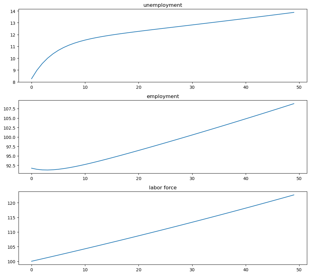
Let’s run a simulation under the default parameters starting from \(X_0 = (12, 138)\).
We will plot the sequences \(\{E_t\}\), \(\{U_t\}\) and \(\{N_t\}\).
N_0 = 150      # Population
e_0 = 0.92     # Initial employment rate
u_0 = 1 - e_0  # Initial unemployment rate
T = 50         # Simulation length

U_0 = u_0 * N_0
E_0 = e_0 * N_0

# Generate X path
X_0 = jnp.array([U_0, E_0])
X_path = generate_path(stock_update, X_0, T, model=model)

# Plot
fig, axes = plt.subplots(3, 1, figsize=(10, 8))
titles = ['unemployment', 'employment', 'labor force']
data = [X_path[0, :], X_path[1, :], X_path.sum(0)]
for ax, title, series in zip(axes, titles, data):
    ax.plot(series, lw=2)
    ax.set_title(title)
plt.tight_layout()
plt.show()
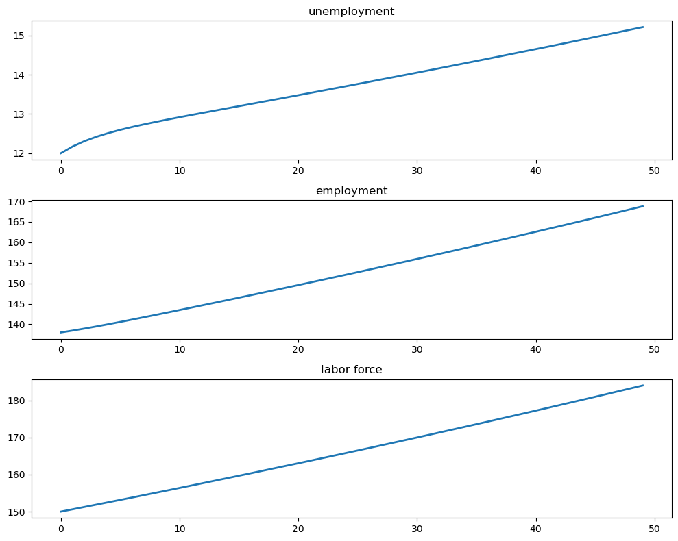
The aggregates \(E_t\) and \(U_t\) don’t converge because their sum \(E_t + U_t\) grows at rate \(g\).
83.3.4. Rate dynamics#
On the other hand, the vector of employment and unemployment rates \(x_t\) can be in a steady state \(\bar x\) if there exists an \(\bar x\) such that
\(\bar x = R \bar x\)
the components satisfy \(\bar e + \bar u = 1\)
This equation tells us that a steady state level \(\bar x\) is an eigenvector of \(R\) associated with a unit eigenvalue.
The following function can be used to compute the steady state.
@jax.jit
def rate_steady_state(model: LakeModel) -> jnp.ndarray:
    r"""
    Finds the steady state of the system :math:`x_{t+1} = R x_{t}`
    by computing the eigenvector corresponding to the largest eigenvalue.

    By the Perron-Frobenius theorem, since :math:`R` is a non-negative
    matrix with columns summing to 1 (a stochastic matrix), the largest
    eigenvalue equals 1 and the corresponding eigenvector gives the steady state.
    """
    λ, α, b, d, A, R, g = model
    eigenvals, eigenvec = jnp.linalg.eig(R)

    # Find the eigenvector corresponding to the largest eigenvalue
    # (which is 1 for a stochastic matrix by Perron-Frobenius theorem)
    max_idx = jnp.argmax(jnp.abs(eigenvals))

    # Get the corresponding eigenvector
    steady_state = jnp.real(eigenvec[:, max_idx])

    # Normalize to ensure positive values and sum to 1
    steady_state = jnp.abs(steady_state)
    steady_state = steady_state / jnp.sum(steady_state)

    return steady_state
We also have \(x_t \to \bar x\) as \(t \to \infty\) provided that the remaining eigenvalue of \(R\) has modulus less than 1.
This is the case for our default parameters:
model = create_lake_model()
e, f = jnp.linalg.eigvals(model.R)
print(f"Eigenvalue magnitudes: {abs(e):.2f}, {abs(f):.2f}")
Eigenvalue magnitudes: 0.70, 1.00
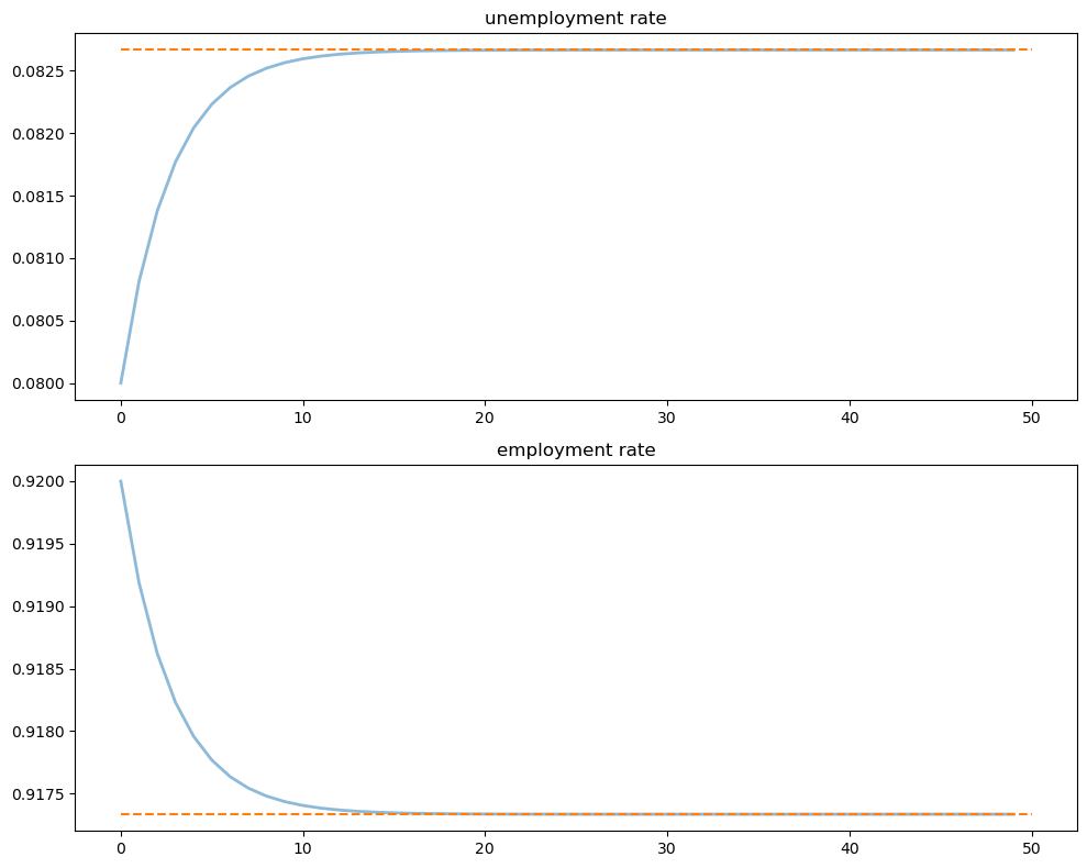
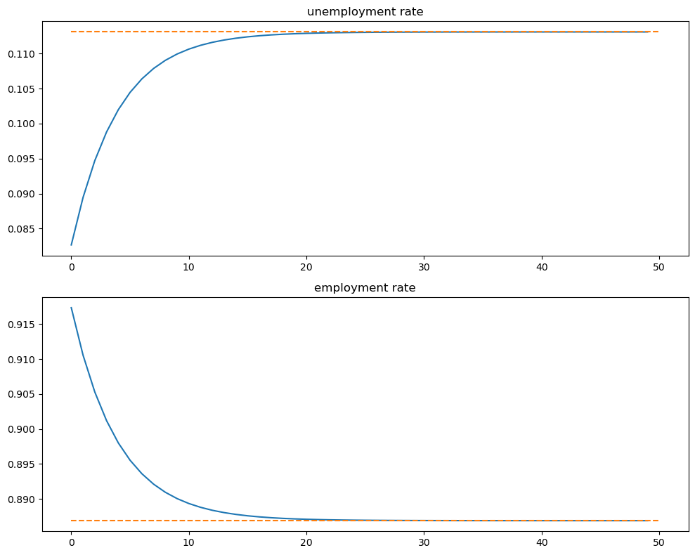
Let’s look at the convergence of the unemployment and employment rates to steady state levels (dashed line)
xbar = rate_steady_state(model)

fig, axes = plt.subplots(2, 1, figsize=(10, 8))
x_0 = jnp.array([u_0, e_0])
x_path = generate_path(rate_update, x_0, T, model=model)

titles = ['unemployment rate', 'employment rate']

for i, title in enumerate(titles):
    axes[i].plot(x_path[i, :], lw=2, alpha=0.5)
    axes[i].hlines(xbar[i], 0, T, color='C1', linestyle='--')
    axes[i].set_title(title)

plt.tight_layout()
plt.show()
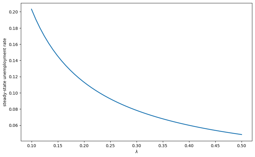
Exercise 83.1
Use JAX’s vmap to compute steady-state unemployment rates for a range of job finding rates \(\lambda\) (from 0.1 to 0.5), and plot the relationship.
Solution
Here is one solution
@jax.jit
def compute_unemployment_rate(λ_val):
    """Computes steady-state unemployment for a given λ"""
    model = create_lake_model(λ=λ_val)
    steady_state = rate_steady_state(model)
    return steady_state[0]

# Use vmap to compute for multiple λ values
λ_values = jnp.linspace(0.1, 0.5, 50)
unemployment_rates = jax.vmap(compute_unemployment_rate)(λ_values)

# Plot the results
fig, ax = plt.subplots(figsize=(10, 6))
ax.plot(λ_values, unemployment_rates, lw=2)
ax.set_xlabel(r'$\lambda$')
ax.set_ylabel('steady-state unemployment rate')
plt.show()
83.4. Dynamics of an individual worker#
An individual worker’s employment dynamics are governed by a finite state Markov process.
The worker can be in one of two states:
\(s_t=0\) means unemployed
\(s_t=1\) means employed
Let’s start off under the assumption that \(b = d = 0\).
The associated transition matrix is then
Let \(\psi_t\) denote the marginal distribution over employment/unemployment states for the worker at time \(t\).
As usual, we regard it as a row vector.
We know from an earlier discussion that \(\psi_t\) follows the law of motion
We also know from the lecture on finite Markov chains that if \(\alpha \in (0, 1)\) and \(\lambda \in (0, 1)\), then \(P\) has a unique stationary distribution, denoted here by \(\psi^*\).
The unique stationary distribution satisfies
Not surprisingly, probability mass on the unemployment state increases with the dismissal rate and falls with the job finding rate.
83.4.1. Ergodicity#
Let’s look at a typical lifetime of employment-unemployment spells.
We want to compute the average amounts of time an infinitely lived worker would spend employed and unemployed.
Let
and
(As usual, \(\mathbb 1\{Q\} = 1\) if statement \(Q\) is true and 0 otherwise)
These are the fraction of time a worker spends unemployed and employed, respectively, up until period \(T\).
If \(\alpha \in (0, 1)\) and \(\lambda \in (0, 1)\), then \(P\) is ergodic, and hence we have
with probability one.
Inspection tells us that \(P\) is exactly the transpose of \(R\) under the assumption \(b=d=0\).
Thus, the percentages of time that an infinitely lived worker spends employed and unemployed equal the fractions of workers employed and unemployed in the steady state distribution.
83.4.2. Convergence rate#
How long does it take for time series sample averages to converge to cross-sectional averages?
We can investigate this by simulating the Markov chain.
Let’s plot the path of the sample averages over 5,000 periods
def markov_update(state, P, key):
    """
    Sample next state from transition probabilities.
    """
    probs = P[state]
    state_new = jax.random.choice(key,
                        a=jnp.arange(len(probs)),
                        p=probs)
    return state_new

model_markov = create_lake_model(d=0, b=0)
T = 5000  # Simulation length

α, λ = model_markov.α, model_markov.λ

P = jnp.array([[1 - λ,        λ],
              [    α,    1 - α]])

xbar = rate_steady_state(model_markov)

# Simulate the Markov chain - we need a different approach for random updates
key = jax.random.PRNGKey(0)

def simulate_markov(P, initial_state, T, key):
    """Simulate Markov chain for T periods"""
    keys = jax.random.split(key, T)

    def scan_fn(state, key):
        next_state = markov_update(state, P, key)
        return next_state, state

    _, path = jax.lax.scan(scan_fn, initial_state, keys)
    return path

s_path = simulate_markov(P, 1, T, key)

fig, axes = plt.subplots(2, 1, figsize=(10, 8))
s_bar_e = jnp.cumsum(s_path) / jnp.arange(1, T+1)
s_bar_u = 1 - s_bar_e

to_plot = [s_bar_u, s_bar_e]
titles = ['percent of time unemployed', 'percent of time employed']

for i, plot in enumerate(to_plot):
    axes[i].plot(plot, lw=2, alpha=0.5)
    axes[i].hlines(xbar[i], 0, T, color='C1', linestyle='--')
    axes[i].set_title(titles[i])

plt.tight_layout()
plt.show()
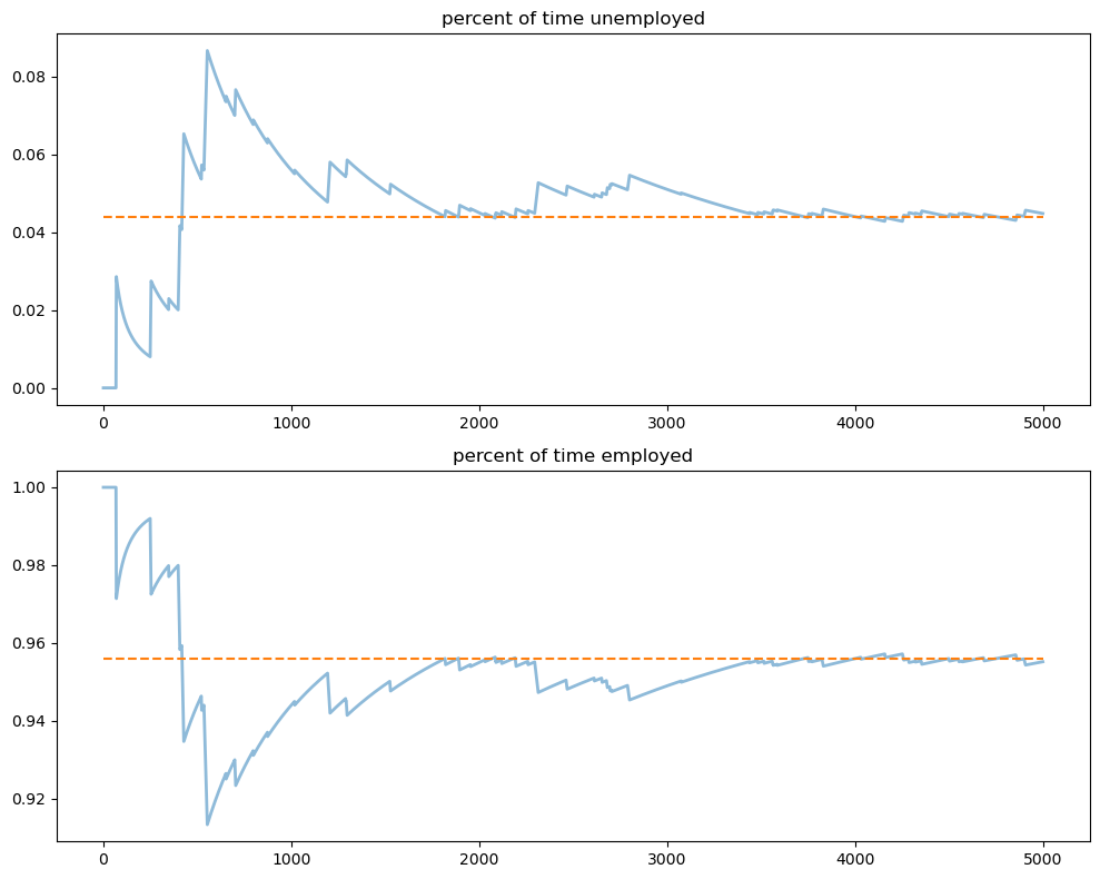
The stationary probabilities are given by the dashed line.
In this case it takes much of the sample for these two objects to converge.
This is largely due to the high persistence in the Markov chain.
83.5. Exercises#
Exercise 83.2
Consider an economy with an initial stock of workers \(N_0 = 100\) at the steady state level of employment in the baseline parameterization.
Suppose that in response to new legislation the hiring rate reduces to \(\lambda = 0.2\).
Plot the transition dynamics of the unemployment and employment stocks for 50 periods.
Plot the transition dynamics for the rates.
How long does the economy take to converge to its new steady state?
What is the new steady state level of employment?
Solution
We begin by constructing the model with default parameters and finding the initial steady state
model_initial = create_lake_model()
x0 = rate_steady_state(model_initial)
print(f"Initial Steady State: {x0}")
Initial Steady State: [0.08266623 0.9173338 ]
Initialize the simulation values
N0 = 100
T = 50
New legislation changes \(\lambda\) to \(0.2\)
model_ex2 = create_lake_model(λ=0.2)
xbar = rate_steady_state(model_ex2)  # new steady state

# Simulate paths
X_path = generate_path(stock_update, x0 * N0, T, model=model_ex2)
x_path = generate_path(rate_update, x0, T, model=model_ex2)
print(f"New Steady State: {xbar}")
New Steady State: [0.11309288 0.8869071 ]
Now plot stocks
fig, axes = plt.subplots(3, 1, figsize=[10, 9])

axes[0].plot(X_path[0, :])
axes[0].set_title('unemployment')

axes[1].plot(X_path[1, :])
axes[1].set_title('employment')

axes[2].plot(X_path.sum(0))
axes[2].set_title('labor force')

plt.tight_layout()
plt.show()
And how the rates evolve
fig, axes = plt.subplots(2, 1, figsize=(10, 8))

titles = ['unemployment rate', 'employment rate']

for i, title in enumerate(titles):
    axes[i].plot(x_path[i, :])
    axes[i].hlines(xbar[i], 0, T, color='C1', linestyle='--')
    axes[i].set_title(title)

plt.tight_layout()
plt.show()
We see that it takes 20 periods for the economy to converge to its new steady state levels.
Exercise 83.3
Consider an economy with an initial stock of workers \(N_0 = 100\) at the steady state level of employment in the baseline parameterization.
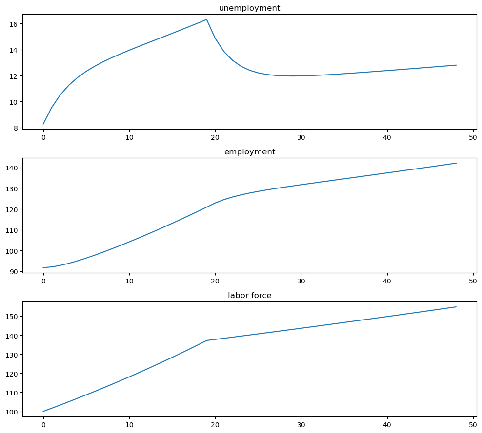
Suppose that for 20 periods the birth rate was temporarily high (\(b = 0.025\)) and then returned to its original level.
Plot the transition dynamics of the unemployment and employment stocks for 50 periods.
Plot the transition dynamics for the rates.
How long does the economy take to return to its original steady state?
Solution
This exercise has the economy experiencing a boom in entrances to the labor market and then later returning to the original levels.
For 20 periods the economy has a new entry rate into the labor market.
Let’s start off at the baseline parameterization and record the steady state
model_baseline = create_lake_model()
x0 = rate_steady_state(model_baseline)
N0 = 100
T = 50
Here are the other parameters:
b_hat = 0.025
T_hat = 20
Let’s increase \(b\) to the new value and simulate for 20 periods
model_high_b = create_lake_model(b=b_hat)

# Simulate stocks and rates for first 20 periods
X_path1 = generate_path(stock_update, x0 * N0, T_hat, model=model_high_b)
x_path1 = generate_path(rate_update, x0, T_hat, model=model_high_b)
Now we reset \(b\) to the original value and then, using the state after 20 periods for the new initial conditions, we simulate for the additional 30 periods
# Use final state from period 20 as initial condition
X_path2 = generate_path(stock_update, X_path1[:, -1], T-T_hat,
                            model=model_baseline)
x_path2 = generate_path(rate_update, x_path1[:, -1], T-T_hat,
                            model=model_baseline)
Finally, we combine these two paths and plot
# Combine paths
X_path = jnp.hstack([X_path1, X_path2[:, 1:]])
x_path = jnp.hstack([x_path1, x_path2[:, 1:]])

fig, axes = plt.subplots(3, 1, figsize=[10, 9])

axes[0].plot(X_path[0, :])
axes[0].set_title('unemployment')

axes[1].plot(X_path[1, :])
axes[1].set_title('employment')

axes[2].plot(X_path.sum(0))
axes[2].set_title('labor force')

plt.tight_layout()
plt.show()
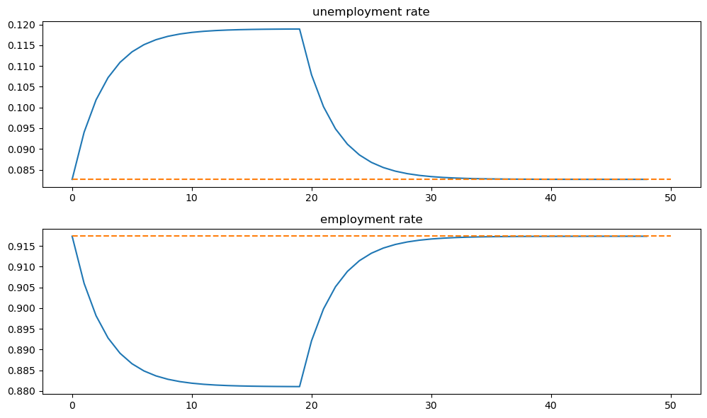
And the rates
fig, axes = plt.subplots(2, 1, figsize=[10, 6])

titles = ['unemployment rate', 'employment rate']

for i, title in enumerate(titles):
    axes[i].plot(x_path[i, :])
    axes[i].hlines(x0[i], 0, T, color='C1', linestyle='--')
    axes[i].set_title(title)

plt.tight_layout()
plt.show()