80. The LQ Permanent Income Model#
80.1. Overview#
This lecture studies consumption smoothing in a linear-quadratic (LQ) permanent income model.
It presents a rational-expectations version of the permanent income theories of Friedman [1956] and Hall [1978].
Throughout, we set \(\beta R = 1\), so that the baseline consumer’s subjective discount factor equals the bond price.
The model is useful for studying
impulse response functions
alternative state-space representations of the optimal decision rule
cointegration of consumption and assets
We derive the consumer’s optimal consumption function, present two state-space representations of the optimal decision rule, and illustrate them with two classic examples.
This is the first of three lectures on the LQ permanent income model.
The two sequels build directly on the tools developed here.
Consumption Smoothing with Incomplete and Complete Markets studies the cross-section behavior of consumption and embeds the single consumer in closed economies with incomplete and complete markets.
Robust Consumption Smoothing and Precautionary Savings studies a consumer who distrusts his model of income and engages in precautionary savings.
Let’s begin with some imports.
import numpy as np
import matplotlib.pyplot as plt
from scipy.linalg import solve, inv, solve_discrete_lyapunov
from scipy.stats import norm
80.2. The standard LQ permanent income model#
80.2.1. Setup#
A consumer has preferences over consumption streams ordered by
where \(\mathbb{E}_t\) is a mathematical expectation conditioned on the consumer’s time-\(t\) information, \(c_t\) is time-\(t\) consumption, \(u(c)\) is a strictly concave one-period utility function, and \(\beta \in (0,1)\) is a discount factor.
The consumer maximizes (80.1) by choosing a plan \(\{c_t, b_{t+1}\}_{t=0}^{\infty}\) subject to the sequence of budget constraints
where \(\{y_t\}\) is an exogenous stationary endowment process, \(R\) is a constant gross risk-free interest rate, \(b_t\) is a one-period risk-free bond maturing at \(t\), and \(b_0\) is a given initial condition.
Note
For \(t \geq 1\), \(b_t\) is chosen at time \(t-1\).
The bond \(b_t > 0\) represents debt owed by the consumer at the start of period \(t\).
We assume \(R^{-1} = \beta\).
The endowment or non-financial income process has the state-space representation
where \(w_{t+1}\) is IID with mean zero and identity covariance matrix, \(\check{A}\) is a stable matrix (eigenvalues strictly less than one in modulus), and \(\check{G}\) is a row vector.
The state confronting the household at \(t\) is \(\bigl[b_t \;\; z_t^\top\bigr]^\top\), where \(b_t\) is its one-period debt due at the start of period \(t\) and \(z_t\) contains all variables useful for forecasting its future endowment.
To make the problem linear-quadratic, we adopt the quadratic utility function
where \(\gamma > 0\) is a bliss level of consumption.
We allow \(c_t\) to be negative (a producer rather than a consumer).
We impose a transversality condition
which rules out Ponzi schemes.
80.2.2. Euler equation and certainty equivalence#
With quadratic utility, the first-order conditions for the consumer’s problem imply that
Note
Equation (80.5) says that consumption is a martingale.
This is the key implication of the LQ permanent income model.
It contrasts with models that have convex marginal utility (\(u''' > 0\)), where consumption is instead a submartingale.
Because the consumer maximizes a quadratic objective subject to a linear transition equation, the problem satisfies a certainty-equivalence property.
This implies that we can find the optimal plan by
first solving the problem while pretending to have perfect foresight; this lets us express \(c_t\) as a function of \(b_t\) and the continuation sequence \(\{y_{t+j}\}_{j=0}^{\infty}\)
then simply replace \(\{y_{t+j}\}_{j=0}^{\infty}\) with \(\{\mathbb{E}_t y_{t+j}\}_{j=0}^{\infty}\).
80.2.3. The optimal consumption function#
Solving the budget constraint (80.2) forward, imposing the transversality condition, and taking conditional expectations gives
Rearranging yields the consumption function
Equivalently, with net interest rate \(r\) defined by \(\beta = 1/(1+r)\),
Evidently, consumption at \(t\) equals \(r/(1+r)\) times total wealth, where total wealth is the sum of human wealth \(\sum_{j=0}^{\infty}\beta^j \mathbb{E}_t y_{t+j}\) and financial wealth \(-b_t\).
Using state-space representation (80.3) to evaluate the geometric sum of expected future endowments,
we obtain
This expresses \(c_t\) as a function of the state \([b_t,\, z_t^\top]^\top\) that confronts the household.
80.2.4. Representation 1: state \((b_t, z_t)\)#
Combining the endowment law of motion with the optimal debt dynamics (derived by substituting (80.10) into (80.2)) gives the following representation:
In this representation the exogenous state is \(z_t\) and the endogenous state is \(b_t\).
We turn now to an alternative representation.
80.2.5. Representation 2: state \((c_t, z_t)\)#
Hall [1978] showed that the LQ permanent income model implies a representation in which the state consists of current consumption \(c_t\) and the exogenous endowment state \(z_t\).
In this representation, \(b_t\) becomes an outcome rather than a state variable.
Shifting (80.7) forward, eliminating \(b_{t+1}\) via (80.2), and rearranging yields
The right-hand side is \((1-\beta)\) times the time-\((t+1)\) innovation to the expected present value of the endowment stream.
Suppose the endowment has the (Wold) moving-average representation
where \(d(L) = \check{G}(I - \check{A} L)^{-1}\check{C}\).
Then
Substituting (80.14) into (80.12) gives the key result
Here, \(d(\beta) = \check{G}(I-\beta\check{A})^{-1}\check{C}\) is the present value of the (Wold) moving-average coefficients.
Thus, consumption is a random walk with innovation \((1-\beta)d(\beta)w_{t+1}\).
Combining (80.15) and (80.6) gives
This representation reveals several important features of the optimal decision rule:
State: The state consists of the endogenous component \(c_t\) and the exogenous component \(z_t\), with financial assets \(b_t\) encoded in \(c_t\) rather than carried as a separate state.
Random walk: Consumption is a random walk with innovation \((1-\beta)d(\beta)w_{t+1}\), which confirms that the Euler equation (80.5) is built into the solution and implies that consumption has no asymptotic stationary distribution.
Box impulse response: For all \(j \geq 1\), the response of \(c_{t+j}\) to the innovation \(w_{t+1}\) is the constant \((1-\beta)d(\beta)\), giving a “box-shaped” impulse response.
Cointegration: Both \(c_t\) and \(b_t\) are nonstationary (unit-root processes), but the linear combination \((1-\beta)b_t + c_t\) is stationary.
From (80.6),
The left side is the cointegrating residual.
80.2.6. Debt dynamics#
Subtracting (80.16) (equation for \(b_t\)) at time \(t\) from the same equation at time \(t+1\) and substituting gives
This shows that \(b_{t+1}\) is predetermined at time \(t\) as a function of \(z_t\) alone.
Solving backward from any \(t\), \(b_t\) depends on the entire history \(z^{t-1} = [z_{t-1},\ldots,z_0]\) and the initial condition \(b_0\).
Such history dependence is a hallmark of a consumption plan in various incomplete-markets economies.
80.2.7. Two classic examples#
We illustrate formulas (80.16) with two examples.
In both, the endowment is \(y_t = z_{1t} + z_{2t}\), where
Here \(z_{1t}\) is a permanent component of \(y_t\) and \(z_{2t}\) is a purely transitory component.
In the full-information example, the consumer observes the state \(z_t\) at time \(t\), so he can reconstruct \(w_{t+1}\) from \(z_{t+1}\) and \(z_t\).
Applying (80.16):
A unit increment to the permanent component \(z_{1t}\) raises consumption one-for-one permanently and causes zero net saving.
A unit increment to the purely transitory component raises consumption by only the fraction \((1-\beta)\) permanently, while the remaining fraction \(\beta\) is saved.
From (80.18):
confirming that none of the permanent shock is saved, while all of the transitory shock is saved.
In the incomplete-information (Muth model) example, the consumer observes \(y_t\) and its history, but not \(z_{1t}\) and \(z_{2t}\) separately.
The appropriate approach uses an innovations representation derived by the Kalman filter.
At the Kalman filter steady state, the Kalman gain \(K \in [0,1]\) satisfies
where \(K\) increases with the ratio \(\sigma_1^2/\sigma_2^2\) (the variance of the permanent shock relative to the transitory shock).
The innovations representation expresses the endowment as an ARMA(1,1) in its own innovation \(a_t = y_t - \mathbb{E}[y_t \mid y^{t-1}]\) (the one-step-ahead forecast error):
Here the coefficient \(-(1-K)\) on the lagged innovation reflects that only the fraction \(K\) of last period’s surprise was treated as permanent; the remainder mean-reverts.
The scalar \(a_t\) is IID with variance \(\Sigma + \sigma_2^2\).
Applying (80.16) to this innovation representation:
The consumer regards a fraction \(K\) of the innovation \(a_{t+1}\) as permanent and fraction \(1-K\) as transitory.
He permanently increments consumption by \(K + (1-\beta)(1-K) = 1 - \beta(1-K)\) of \(a_{t+1}\) and saves the remaining fraction \(\beta(1-K)\).
The first difference of income obeys a first-order moving average:
By contrast, the first difference of consumption is IID by (80.24).
80.2.8. Implementation#
# Parameters
β = 0.95       # discount factor (so R = 1/β)
σ1 = 0.15      # std of permanent shock
σ2 = 0.30      # std of transitory shock

# Example 1: full information
A_check = np.array([[1.0, 0.0],
                    [0.0, 0.0]])
C_check = np.array([[σ1, 0.0],
                    [0.0, σ2]])
G_check = np.array([[1.0, 1.0]])

# Key matrix M = G(I - βA)^{-1}
IbA = np.eye(2) - β * A_check
M = G_check @ inv(IbA)   # shape (1, 2)

# Consumption impulse responses
h = (1 - β) * M @ C_check          # shape (1, 2)
irf_perm_ex1 = h[0, 0] / σ1       # response per unit std of permanent shock
irf_trans_ex1 = h[0, 1] / σ2       # response per unit std of transitory shock

print("Example 1 (full information)")
print(f"  IRF c to permanent shock  (normalised): {irf_perm_ex1:.4f}   "
      f"(theory: 1.0)")
print(f"  IRF c to transitory shock (normalised): {irf_trans_ex1:.4f}   "
      f"(theory: {1-β:.4f})")
Example 1 (full information)
  IRF c to permanent shock  (normalised): 1.0000   (theory: 1.0)
  IRF c to transitory shock (normalised): 0.0500   (theory: 0.0500)
# Example 2: partial information
Σ = (σ1**2 + np.sqrt(σ1**4 + 4 * σ1**2 * σ2**2)) / 2
K = Σ / (Σ + σ2**2)

print("Example 2 (partial information)")
print(f"  Steady-state Kalman gain K = {K:.4f}")
print(f"  IRF c to unit innovation a_{{t+1}}: {1 - β*(1-K):.4f}")
print(f"  Fraction of innovation treated as permanent (K): {K:.4f}")
print(f"  Fraction saved: β(1-K) = {β*(1-K):.4f}")
Example 2 (partial information)
  Steady-state Kalman gain K = 0.3904
  IRF c to unit innovation a_{t+1}: 0.4209
  Fraction of innovation treated as permanent (K): 0.3904
  Fraction saved: β(1-K) = 0.5791
# Compare impulse responses
T = 30
irf_c_ex1_perm = np.ones(T) * irf_perm_ex1 * σ1
irf_c_ex1_trans = np.ones(T) * irf_trans_ex1 * σ2

irf_c_ex2 = np.ones(T) * (1 - β * (1 - K))   # per unit innovation a_t

fig, axes = plt.subplots(1, 2, figsize=(12, 4))

axes[0].axhline(0, color='k', linewidth=0.8)
axes[0].step(range(T), irf_c_ex1_perm, where='post',
             label='permanent shock ($z_1$)', color='C0', lw=2)
axes[0].step(range(T), irf_c_ex1_trans, where='post',
             label='transitory shock ($z_2$)', color='C3',
             linestyle='--', lw=2)
axes[0].set_xlabel('periods after shock')
axes[0].set_ylabel('response of $c$')
axes[0].set_title('full information')
axes[0].legend()

axes[1].axhline(0, color='k', linewidth=0.8)
axes[1].step(range(T), irf_c_ex2, where='post',
             label=f'unit innovation $a_{{t+1}}$ (K = {K:.2f})',
             color='C4', lw=2)
axes[1].set_xlabel('periods after shock')
axes[1].set_ylabel('response of $c$')
axes[1].set_title('partial information')
axes[1].legend()
fig.tight_layout()
plt.show()
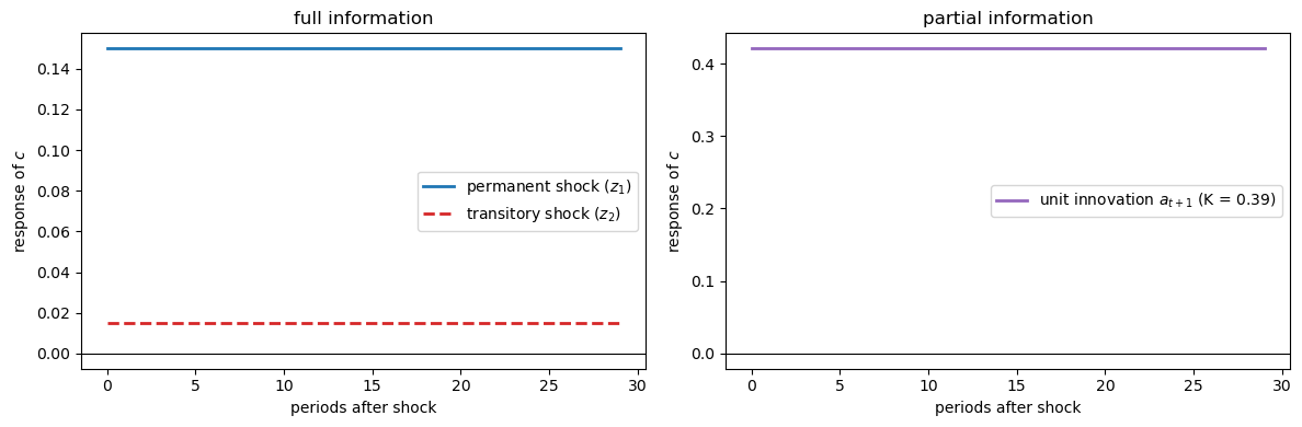
Fig. 80.1 Consumption impulse responses#
Note
The impulse responses have the “box” shape characteristic of the LQ permanent income model: once a shock occurs, consumption shifts permanently to a new level and stays there.
The two representations and examples developed here are the foundation for the two sequel lectures.
Consumption Smoothing with Incomplete and Complete Markets uses the \((c_t, z_t)\) representation (80.16) to study how the cross-section distribution of consumption evolves in closed economies with incomplete and complete markets.
Robust Consumption Smoothing and Precautionary Savings studies a consumer who distrusts the endowment process (80.3) and engages in precautionary savings.
80.3. Exercises#
Exercise 80.1
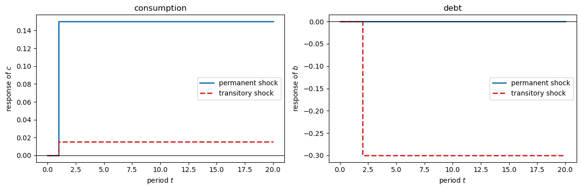
This exercise verifies the response of consumption and debt to permanent and transitory shocks in the full-information two-factor model.
Consider the model of (80.19) with the calibration used above.
Suppose the economy starts at \(z_0 = 0\) and \(b_0 = 0\) and is hit by a single shock at \(t = 1\): either a unit permanent shock \(w_1 = (1, 0)^\top\) or a unit transitory shock \(w_1 = (0, 1)^\top\), with no further shocks thereafter.
Using representation (80.11), compute and plot the paths of consumption \(c_t\) and debt \(b_t\) following each shock.
Confirm that the permanent shock raises consumption permanently by \(\sigma_1\) and induces no saving, while the transitory shock raises consumption permanently by \((1-\beta)\sigma_2\) and is otherwise saved.
Solution
Here is one solution:
We iterate representation (80.11) forward with a single shock at \(t = 1\).
def impulse_response(shock, T=20):
    """Paths of c and b after a single shock at t=1 (z_0 = b_0 = 0)."""
    I2 = np.eye(2)
    b_coef = M @ (A_check - I2)      # coefficient on z_t in the b law

    z = np.zeros((T + 1, 2))
    b = np.zeros(T + 1)

    z[1] = C_check @ shock           # shock realized at t = 1
    for t in range(1, T):
        z[t + 1] = A_check @ z[t]
    for t in range(T):
        b[t + 1] = b[t] + (b_coef @ z[t]).item()

    c = np.array([((1 - β) * (M @ z[t] - b[t])).item() for t in range(T + 1)])
    return c, b


c_perm, b_perm = impulse_response(np.array([1.0, 0.0]))
c_tran, b_tran = impulse_response(np.array([0.0, 1.0]))

fig, axes = plt.subplots(1, 2, figsize=(12, 4))

axes[0].step(range(len(c_perm)), c_perm, where='post',
             label='permanent shock', color='C0', lw=2)
axes[0].step(range(len(c_tran)), c_tran, where='post',
             label='transitory shock', color='C3', linestyle='--', lw=2)
axes[0].axhline(0, color='k', lw=0.8)
axes[0].set_xlabel('period $t$')
axes[0].set_ylabel('response of $c$')
axes[0].set_title('consumption')
axes[0].legend()

axes[1].step(range(len(b_perm)), b_perm, where='post',
             label='permanent shock', color='C0', lw=2)
axes[1].step(range(len(b_tran)), b_tran, where='post',
             label='transitory shock', color='C3', linestyle='--', lw=2)
axes[1].axhline(0, color='k', lw=0.8)
axes[1].set_xlabel('period $t$')
axes[1].set_ylabel('response of $b$')
axes[1].set_title('debt')
axes[1].legend()
fig.tight_layout()
plt.show()

print(f"permanent shock:  Δc = {c_perm[-1]:.4f}  (theory σ1 = {σ1:.4f}),"
      f"  Δb = {b_perm[-1]:.4f}")
print(f"transitory shock: Δc = {c_tran[-1]:.4f}  "
      f"(theory (1-β)σ2 = {(1-β)*σ2:.4f}),  Δb = {b_tran[-1]:.4f}")
permanent shock:  Δc = 0.1500  (theory σ1 = 0.1500),  Δb = 0.0000
transitory shock: Δc = 0.0150  (theory (1-β)σ2 = 0.0150),  Δb = -0.3000
The permanent shock lifts consumption by \(\sigma_1\) and leaves debt at zero: the shock is fully capitalised, so there is no net saving.
The transitory shock lifts consumption by only \((1-\beta)\sigma_2\); the consumer saves the remainder, so debt falls to \(-\sigma_2\) (assets accumulate).
Exercise 80.2
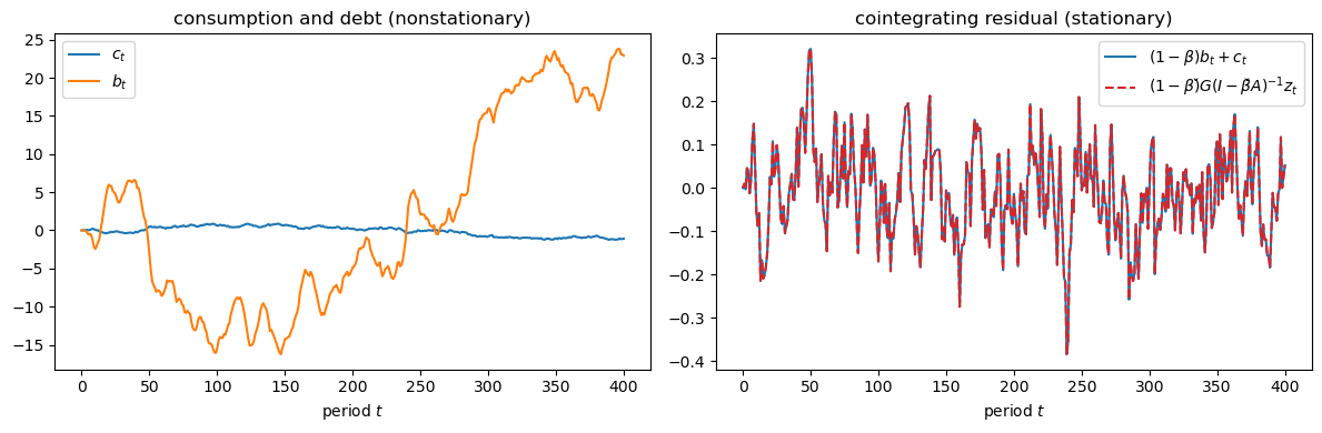
This exercise illustrates the cointegration of consumption and debt described in (80.17).
The cointegration result requires a stationary endowment, so we replace the two-factor process with a scalar AR(1),
with \(\rho = 0.7\) and \(\sigma_\varepsilon = 0.5\).
Simulate a long path of \(c_t\) and \(b_t\) using representation (80.11).
Verify that \(c_t\) and \(b_t\) each inherit a unit root (they wander), while the cointegrating residual \((1-\beta)b_t + c_t\) is stationary and equals \((1-\beta)\check{G}(I-\beta\check{A})^{-1}z_t\).
Solution
Here is one solution:
ρ, σε = 0.7, 0.5
A_ar = np.array([[ρ]])
C_ar = np.array([[σε]])
G_ar = np.array([[1.0]])

M_ar = G_ar @ inv(np.eye(1) - β * A_ar)     # G(I - βA)^{-1}
b_coef_ar = M_ar @ (A_ar - np.eye(1))       # coefficient on z_t in b law

rng = np.random.default_rng(0)
T = 400
z = np.zeros((T + 1, 1))
b = np.zeros(T + 1)
for t in range(T):
    z[t + 1] = A_ar @ z[t] + C_ar @ rng.standard_normal(1)
    b[t + 1] = b[t] + (b_coef_ar @ z[t]).item()

c = np.array([((1 - β) * (M_ar @ z[t] - b[t])).item() for t in range(T + 1)])
residual = (1 - β) * b + c
theory = np.array([((1 - β) * (M_ar @ z[t])).item() for t in range(T + 1)])

fig, axes = plt.subplots(1, 2, figsize=(12, 4))
axes[0].plot(c, label='$c_t$', lw=1.5)
axes[0].plot(b, label='$b_t$', lw=1.5)
axes[0].set_xlabel('period $t$')
axes[0].set_title('consumption and debt (nonstationary)')
axes[0].legend()

axes[1].plot(residual, label=r'$(1-\beta)b_t + c_t$', lw=1.5, color='C0')
axes[1].plot(theory, label=r'$(1-\beta)\check{G}(I-\beta\check{A})^{-1}z_t$',
             lw=1.5, linestyle='--', color='C3')
axes[1].set_xlabel('period $t$')
axes[1].set_title('cointegrating residual (stationary)')
axes[1].legend()
fig.tight_layout()
plt.show()

print(f"max |residual - theory| = {np.max(np.abs(residual - theory)):.2e}")
max |residual - theory| = 2.36e-16
Both \(c_t\) and \(b_t\) inherit the unit root that the random-walk consumption rule builds into the solution, so they drift without settling down.
Their linear combination \((1-\beta)b_t + c_t\) coincides with \((1-\beta)\check{G}(I-\beta\check{A})^{-1}z_t\) (up to floating-point error), which is a stationary function of the stationary state \(z_t\).
Exercise 80.3
This exercise explores how the consumer’s information problem shapes his response to income surprises in the Muth model.
Recall from (80.24) that the permanent consumption response to a unit income innovation \(a_{t+1}\) is \(1 - \beta(1-K)\), where the Kalman gain \(K\) in (80.22) depends on the ratio \(\sigma_1/\sigma_2\).
Plot the response \(1 - \beta(1-K)\) as a function of the ratio \(\sigma_1/\sigma_2\), holding \(\sigma_2\) fixed.
Explain the two limiting cases \(\sigma_1/\sigma_2 \to 0\) and \(\sigma_1/\sigma_2 \to \infty\), and relate them to the two shocks of the full-information model.
Solution
Here is one solution:
ratios = np.linspace(0.02, 6.0, 300)
σ2_fixed = 0.30

responses = []
for r in ratios:
    s1 = r * σ2_fixed
    Σ = (s1**2 + np.sqrt(s1**4 + 4 * s1**2 * σ2_fixed**2)) / 2
    K = Σ / (Σ + σ2_fixed**2)
    responses.append(1 - β * (1 - K))

fig, ax = plt.subplots()
ax.plot(ratios, responses, lw=2, color='C0')
ax.axhline(1.0, color='C3', linestyle='--', lw=1,
           label=r'permanent limit ($K\to1$)')
ax.axhline(1 - β, color='C4', linestyle='--', lw=1,
           label=r'transitory limit ($K\to0$): $1-\beta$')
ax.set_xlabel(r'$\sigma_1/\sigma_2$')
ax.set_ylabel(r'consumption response $1-\beta(1-K)$')
ax.legend()
plt.show()
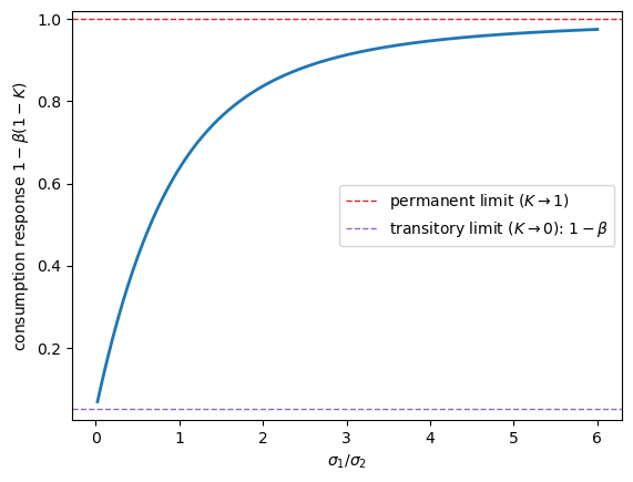
As \(\sigma_1/\sigma_2 \to 0\) the endowment is dominated by transitory noise, so \(K \to 0\): the consumer treats each innovation as transitory and raises consumption by only \(1-\beta\), exactly as for the purely transitory shock in the full-information model.
As \(\sigma_1/\sigma_2 \to \infty\) the endowment is dominated by permanent shocks, so \(K \to 1\): the consumer treats each innovation as permanent and raises consumption one-for-one, exactly as for the permanent shock.
For intermediate ratios the consumer optimally splits each surprise, capitalising the fraction \(K\) he attributes to the permanent component and saving the rest.