19. Posterior Distributions for AR(1) Parameters#
GPU
This lecture was built using a machine with access to a GPU — although it will also run without one.
Google Colab has a free tier with GPUs that you can access as follows:
Click on the “play” icon top right
Select Colab
Set the runtime environment to include a GPU
In addition to what’s included in base Anaconda, this lecture requires the following libraries.
We first install numpyro and jax:
!pip install numpyro jax
We also install arviz and pymc:
!pip install arviz pymc
19.1. Overview#
This lecture uses Bayesian methods offered by pymc and numpyro to make statistical inferences about two parameters of a univariate first-order autoregression.
The model is a good laboratory for illustrating consequences of alternative ways of modeling the distribution of the initial \(y_0\):
As a fixed number
As a random variable drawn from the stationary distribution of the \(\{y_t\}\) stochastic process
19.1.1. Setting#
The first component of the statistical model is
where
the scalars \(\rho\) and \(\sigma_x\) satisfy \(|\rho| < 1\) and \(\sigma_x > 0\)
\(\{\epsilon_{t+1}\}\) is a sequence of IID normal random variables with mean \(0\) and variance \(1\).
The second component of the statistical model is
Unknown parameters are \(\rho, \sigma_x\).
We have independent prior probability distributions for \(\rho, \sigma_x\) and want to compute a posterior probability distribution after observing a sample \(\{y_{t}\}_{t=0}^T\).
We want to study how inferences about the unknown parameters \((\rho, \sigma_x)\) depend on what is assumed about the parameters \(\mu_0, \sigma_0\) of the distribution of \(y_0\).
We study two assumptions about the initial value \(y_0\), and we refer to them by name throughout the lecture.
Under the conditioning assumption we take the observed \(y_0\) as given.
Formally we set \((\mu_0, \sigma_0) = (y_0, 0)\), so the density of \(y_0\) is a spike at its observed value.
This density does not depend on \(\rho\) or \(\sigma_x\), so \(y_0\) carries no information about the parameters; in effect we condition on \(y_0\) and model only what happens after it.
Under the stationary assumption we treat \(y_0\) as a draw from the stationary distribution of the process,
This density does depend on \(\rho\) and \(\sigma_x\), so now the observed \(y_0\) carries information about the parameters.
The whole lecture is about how this one difference affects our estimates.
Note
We do not treat a third possible case in which \(\mu_0, \sigma_0\) are free parameters to be estimated.
19.1.2. Libraries#
We use PyMC and NumPyro to compute the posterior distribution of \(\rho, \sigma_x\).
We use two libraries because they make different trade-offs.
PyMC offers a mature and highly readable modeling syntax together with a rich set of diagnostic tools, which makes it convenient for learning and prototyping.
NumPyro is built on JAX, so it compiles to fast machine code and can run on a GPU, which helps it scale to larger models and datasets.
Because both libraries fit the same model, running them side by side also lets us check that they agree.
Both libraries support the NUTS sampler, which we use to draw samples from the posterior.
We treat NUTS as a black box here; see the introduction to NUTS in Non-Conjugate Priors for a brief account of how it works.
19.1.3. Imports#
Let’s start with some Python imports.
import arviz as az
import pymc as pm
import numpyro
from numpyro import distributions as dist

import numpy as np
import jax.numpy as jnp
from jax import random
import matplotlib.pyplot as plt

import logging
logging.basicConfig()
logger = logging.getLogger('pymc')
logger.setLevel(logging.CRITICAL)
19.2. Estimation#
Let’s turn to estimation, starting with the likelihood function.
19.2.1. Likelihood function#
For a sample \(\{y_t\}_{t=0}^T\) from the AR(1) model, the likelihood function can be factored as follows:
(We use \(f\) to denote a generic probability density.)
The statistical model (19.1)-(19.2) implies
We shall use Bayes’ law to construct a posterior distribution under the alternative assumptions.
As discussed above, the way that we select the initial value \(y_0\) matters.
If we believe \(y_0\) really is a draw from the stationary distribution, the stationary assumption is a good choice, because then \(y_0\) carries useful information about \(\rho\) and \(\sigma_x\).
If we suspect \(y_0\) is far out in the tail — so that early observations carry a large transient component — the conditioning assumption is better.
To illustrate the issue, we’ll begin by choosing an initial \(y_0\) that is far out in a tail of the stationary distribution.
19.2.2. Simulation code#
We will work with simulated data, fixing parameters \(\rho\) and \(\sigma_x\).
Then we will pretend that we don’t know these parameters and try to estimate them under the two assumptions discussed above (conditioning and stationary).
The following function simulates a path of the AR(1) process from a given initial condition.
def ar1_simulate(ρ, σ, y0, T, rng):

    # Allocate space and draw shocks
    y = np.empty(T)
    ε = rng.normal(0, σ, T)

    # Initial condition and step forward
    y[0] = y0
    for t in range(1, T):
        y[t] = ρ * y[t-1] + ε[t]

    return y
We use the following parameterization.
σ_true = 1.0   # Fix a value for σ_x
ρ_true = 0.5   # Fix a value for ρ
Our simulated time series will be relatively short, so that the priors matter:
T = 50 # Length of time series
As mentioned above, we choose an initial \(y_0\) that is far out in a tail of the stationary distribution:
y_0 = 10
Now let’s simulate and generate our data:
rng = np.random.default_rng(42)
y = ar1_simulate(ρ_true, σ_true, y_0, T, rng)
Here’s a plot of the simulated series.
fig, ax = plt.subplots()
ax.plot(y, lw=2)
ax.set_xlabel('time')
plt.show()
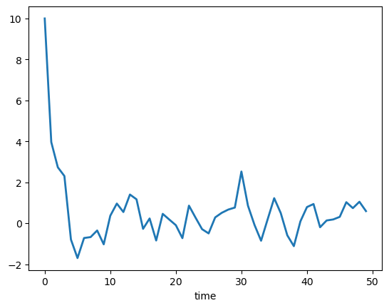
You can see that the initial condition is unusually large — the series moves away from it quickly and fluctuates in a lower band.
19.2.3. PyMC implementation#
In this section we use PyMC to compute the posterior under each assumption about \(y_0\) — first the conditioning assumption, then the stationary assumption.
We parameterize each normal distribution in PyMC by its standard deviation \(\sigma\), via the sigma argument.
AR1_model = pm.Model()

with AR1_model:

    # Start with priors
    ρ = pm.Uniform('rho', lower=-1., upper=1.)  # Assume stable ρ
    σ = pm.HalfNormal('sigma', sigma=np.sqrt(10))

    # Expected value of y at the next period (ρ * y)
    yhat = ρ * y[:-1]

    # Likelihood of the actual realization
    y_like = pm.Normal('y_obs', mu=yhat, sigma=σ, observed=y[1:])
Let’s unpack what this model declares.
Inside the with AR1_model: block, each pm statement adds a random variable to the model.
The first two lines are the priors — a uniform prior on \(\rho\) over \((-1, 1)\), which builds in stationarity, and a half-normal prior on \(\sigma\).
The line yhat = ρ * y[:-1] is just the vector of conditional means \(\rho y_{t-1}\) for \(t = 1, \ldots, T\).
The last line is the likelihood: the keyword observed=y[1:] tells PyMC that the values y[1:] are data, drawn from \(N(\rho y_{t-1}, \sigma^2)\).
Because yhat and y[1:] are whole vectors, this single line encodes the entire product \(\prod_{t=1}^{T} f(y_t \mid y_{t-1})\) from the factorization above.
PyMC multiplies this likelihood by the priors to form the posterior, which we sample from below.
Note
Notice what is absent: we never write down a density for \(y_0\) itself.
It enters the model only inside y[:-1], as the conditioning value for the first transition \(f(y_1 \mid y_0)\) — never as something the model has to explain.
Leaving out the \(f(y_0)\) factor in this way is precisely the conditioning assumption.
pm.sample by default uses the NUTS sampler to generate samples, as shown in the cell below:
with AR1_model:
    trace = pm.sample(50000, tune=10000, return_inferencedata=True)
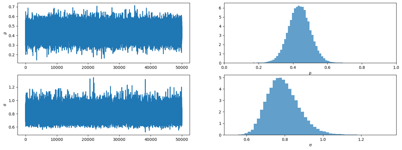
We plot the trace and the posterior densities for the two parameters.
with AR1_model:
    az.plot_trace(trace)
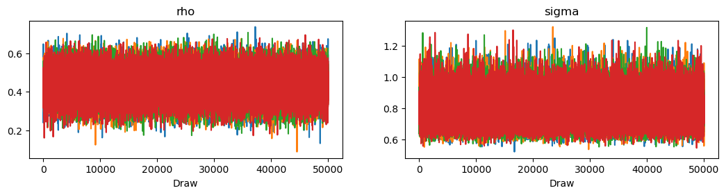
Recall that we generated the data with \(\rho = 0.5\) and \(\sigma_x = 1\).
The posteriors concentrate near these values, so conditioning on \(y_0\) recovers the parameters reasonably well, even from this short sample.
Note
The fit is good but not exact — the posterior for \(\rho\) sits a little below its true value.
This is partly the classic Hurwicz bias: in a first-order autoregression the least-squares (and hence posterior) estimate of \(\rho\) is biased downward in small samples, with the bias shrinking as the sample grows (see Hurwicz [1950] and [Orcutt and Winokur, 1969]).
Here is a numerical summary of the posterior.
with AR1_model:
    summary = az.summary(trace, round_to=4)

summary
| mean | sd | eti89_lb | eti89_ub | ess_bulk | ess_tail | r_hat | mcse_mean | mcse_sd | |
|---|---|---|---|---|---|---|---|---|---|
| rho | 0.4373 | 0.0632 | 0.3366 | 0.5378 | 178483.7049 | 129725.5309 | 1.0 | 0.0001 | 0.0001 |
| sigma | 0.7927 | 0.0835 | 0.6717 | 0.9361 | 179089.7725 | 137719.2218 | 1.0 | 0.0002 | 0.0002 |
Now we switch to the stationary assumption, using the same data.
Recall that this means
We alter the code as follows:
AR1_model_y0 = pm.Model()

with AR1_model_y0:

    # Start with priors
    ρ = pm.Uniform('rho', lower=-1., upper=1.)  # Assume stable ρ
    σ = pm.HalfNormal('sigma', sigma=np.sqrt(10))

    # Standard deviation of the stationary distribution
    y_sd = σ / np.sqrt(1 - ρ**2)

    # Expected value of y at the next period (ρ * y)
    yhat = ρ * y[:-1]
    y_data = pm.Normal('y_obs', mu=yhat, sigma=σ, observed=y[1:])

    # Density for y0 -- this term imposes the stationary assumption
    y0_data = pm.Normal('y0_obs', mu=0., sigma=y_sd, observed=y[0])
The only change from the first model is that final line.
Note
The new line adds a density for \(y_0\) — the stationary density \(N\!\left(0, \sigma_x^2/(1-\rho^2)\right)\) — through a second observed term.
This restores the \(f(y_0)\) factor we dropped before, and so is the stationary assumption.
Everything else is identical, so any difference between the two posteriors comes entirely from this one term.
As before, we sample from the posterior.
with AR1_model_y0:
    trace_y0 = pm.sample(50000, tune=10000, return_inferencedata=True)
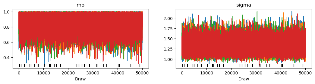
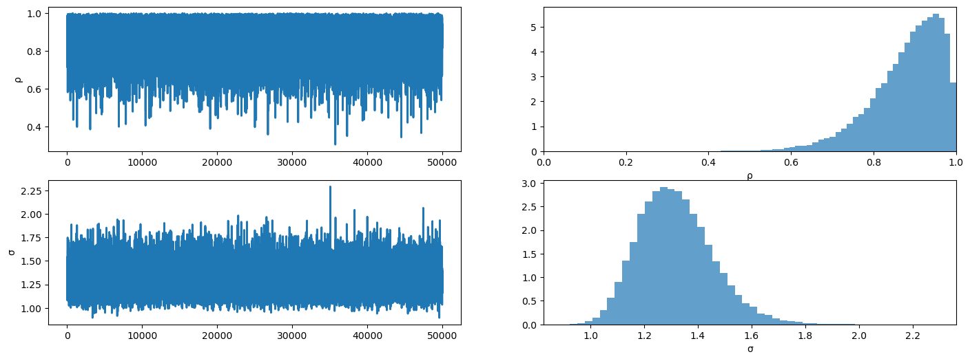
In the trace plot below, any grey vertical lines mark sampler divergences.
with AR1_model_y0:
    az.plot_trace(trace_y0)
Here is a summary of the posterior.
with AR1_model_y0:
    summary_y0 = az.summary(trace_y0, round_to=4)

summary_y0
| mean | sd | eti89_lb | eti89_ub | ess_bulk | ess_tail | r_hat | mcse_mean | mcse_sd | |
|---|---|---|---|---|---|---|---|---|---|
| rho | 0.8796 | 0.0851 | 0.7215 | 0.9819 | 114272.7131 | 88960.5557 | 1.0 | 0.0002 | 0.0002 |
| sigma | 1.3174 | 0.1382 | 1.1168 | 1.5541 | 116064.0531 | 98411.3288 | 1.0 | 0.0004 | 0.0003 |
The posterior for \(\rho\) has clearly moved when we changed our assumption about \(y_0\).
19.2.4. Comparing the two posteriors#
Let’s put the two posteriors for \(\rho\) side by side to see what changed.
The figure below overlays the posterior for \(\rho\) under each assumption, with the true value marked by a dashed line.
ρ_cond = trace.posterior['rho'].values.flatten()
ρ_stat = trace_y0.posterior['rho'].values.flatten()

fig, ax = plt.subplots()
ax.hist(ρ_cond, bins=50, density=True, alpha=0.5,
        label='conditioning assumption')
ax.hist(ρ_stat, bins=50, density=True, alpha=0.5,
        label='stationary assumption')
ax.axvline(ρ_true, color='k', linestyle='--', lw=2, label='true value')
ax.set_xlabel('ρ')
ax.legend()
plt.show()
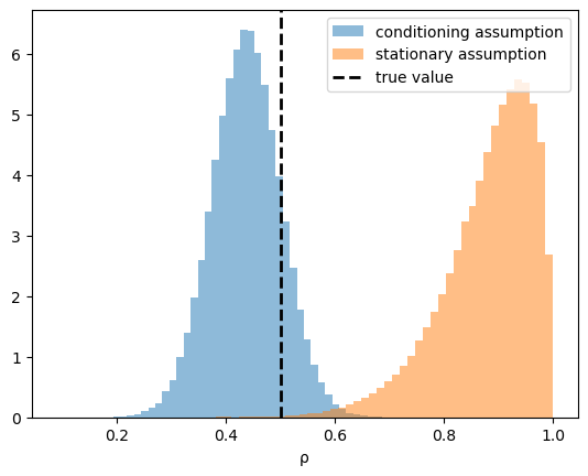
The posterior from the conditioning assumption sits close to the true value of \(0.5\).
It is centred a little below \(0.5\), which is the small-sample Hurwicz bias mentioned above — a mild downward pull that shrinks as the sample grows.
The posterior from the stationary assumption is different: it is pushed well to the right, toward \(\rho = 1\).
Here is why.
We chose a starting value \(y_0 = 10\) that lies far out in the tail of the stationary distribution.
If \(y_0\) really were a draw from that distribution, such an extreme value would be very unlikely.
So when we force the model to explain \(y_0\) this way, Bayes’ law looks for parameter values that make the extreme \(y_0\) plausible.
It does this by pushing \(\rho\) toward \(1\), because a larger \(\rho\) inflates the stationary variance \(\sigma_x^2 / (1 - \rho^2)\) and makes a large \(y_0\) less surprising.
A single unusual starting value therefore drags the whole posterior away from the truth.
This is the sense in which the conditioning assumption is more accurate here: it does not let one atypical observation distort our view of \(\rho\) and \(\sigma_x\).
19.2.5. NumPyro implementation#
We now redo both computations with NumPyro.
Because it fits the same two models, we expect its posteriors to match those from PyMC.
The models are the same; only the syntax differs.
NumPyro describes a model as an ordinary Python function rather than a with block, each numpyro.sample('name', distribution) plays the role that a pm random variable did above, and the keyword obs= is NumPyro’s counterpart of PyMC’s observed=.
Everything we said about priors, the vectorized likelihood, and how the two assumptions are imposed carries over unchanged; see Non-Conjugate Priors for a fuller introduction to NumPyro models.
We start with a helper function that plots the trace and posterior histogram for the sampled parameters.
def plot_posterior(sample):
    """
    Plot trace and histogram
    """
    # To np array
    ρs = np.array(sample['rho'])
    σs = np.array(sample['sigma'])

    fig, axs = plt.subplots(2, 2, figsize=(17, 6))
    # Plot trace
    axs[0, 0].plot(ρs, lw=2)
    axs[1, 0].plot(σs, lw=2)

    # Plot posterior
    axs[0, 1].hist(ρs, bins=50, density=True, alpha=0.7)
    axs[0, 1].set_xlim([0, 1])
    axs[1, 1].hist(σs, bins=50, density=True, alpha=0.7)

    axs[0, 0].set_ylabel('ρ')
    axs[1, 0].set_ylabel('σ')
    axs[0, 1].set_xlabel('ρ')
    axs[1, 1].set_xlabel('σ')
    plt.show()
The first model uses the conditioning assumption.
def AR1_model(data):
    # Set prior
    ρ = numpyro.sample('rho', dist.Uniform(low=-1., high=1.))
    σ = numpyro.sample('sigma', dist.HalfNormal(scale=np.sqrt(10)))

    # Expected value of y at the next period (ρ * y)
    yhat = ρ * data[:-1]

    # Likelihood of the actual realization
    y_data = numpyro.sample('y_obs', dist.Normal(loc=yhat, scale=σ), obs=data[1:])
We convert the data to a JAX array, build the NUTS sampler, and run MCMC.
# Make jnp array
y = jnp.array(y)

# Set NUTS kernel
NUTS_kernel = numpyro.infer.NUTS(AR1_model)

# Run MCMC
mcmc = numpyro.infer.MCMC(NUTS_kernel, num_samples=50000, num_warmup=10000, progress_bar=False)
mcmc.run(rng_key=random.PRNGKey(1), data=y)
We plot the trace and posterior.
plot_posterior(mcmc.get_samples())
Here is the posterior summary.
mcmc.print_summary()
                mean       std    median      5.0%     95.0%     n_eff     r_hat
       rho      0.44      0.06      0.44      0.33      0.54  33558.19      1.00
     sigma      0.79      0.08      0.79      0.66      0.93  32561.73      1.00

Number of divergences: 0
Next we use the stationary assumption, where
Here’s the new code to achieve this.
def AR1_model_y0(data):
    # Set prior
    ρ = numpyro.sample('rho', dist.Uniform(low=-1., high=1.))
    σ = numpyro.sample('sigma', dist.HalfNormal(scale=np.sqrt(10)))

    # Standard deviation of the stationary distribution
    y_sd = σ / jnp.sqrt(1 - ρ**2)

    # Expected value of y at the next period (ρ * y)
    yhat = ρ * data[:-1]

    # Likelihood of the actual realization
    y_data = numpyro.sample('y_obs', dist.Normal(loc=yhat, scale=σ), obs=data[1:])

    # Density for y0 -- this term imposes the stationary assumption
    y0_data = numpyro.sample('y0_obs', dist.Normal(loc=0., scale=y_sd), obs=data[0])
We build the sampler for this model and run MCMC.
# Set NUTS kernel
NUTS_kernel = numpyro.infer.NUTS(AR1_model_y0)

# Run MCMC
mcmc2 = numpyro.infer.MCMC(NUTS_kernel, num_samples=50000, num_warmup=10000, progress_bar=False)
mcmc2.run(rng_key=random.PRNGKey(1), data=y)
Again we plot the trace and posterior.
plot_posterior(mcmc2.get_samples())
And here is the posterior summary.
mcmc2.print_summary()
                mean       std    median      5.0%     95.0%     n_eff     r_hat
       rho      0.88      0.09      0.90      0.76      1.00  32784.94      1.00
     sigma      1.32      0.14      1.31      1.09      1.53  24454.89      1.00

Number of divergences: 0
As with PyMC, the posterior for \(\rho\) shifts toward \(1\) once we switch to the stationary assumption.
To confirm that the two libraries agree, we overlay their posteriors for \(\rho\) under the conditioning assumption.
ρ_pymc = trace.posterior['rho'].values.flatten()
ρ_numpyro = np.array(mcmc.get_samples()['rho'])

fig, ax = plt.subplots()
ax.hist(ρ_pymc, bins=50, density=True, alpha=0.5, label='PyMC')
ax.hist(ρ_numpyro, bins=50, density=True, alpha=0.5, label='NumPyro')
ax.set_xlabel('ρ')
ax.legend()
plt.show()
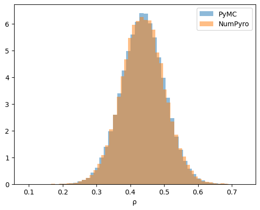
The two posteriors line up, as they should.
19.3. Conclusion#
This lecture showed that what we assume about the initial value \(y_0\) can have a large effect on our estimates of an AR(1) process.
When the sample is short and \(y_0\) might be unusual, the conditioning assumption is the safer choice.
It lets the data speak about \(\rho\) and \(\sigma_x\) without forcing the model to explain the starting value.
The stationary assumption adds information, and that information is valuable when the assumption is true.
But when \(y_0\) is in fact far from typical, the same assumption misleads us — here it pushed \(\rho\) toward \(1\) and away from the truth.
A simple rule of thumb:
use the conditioning assumption when early observations look transient or the starting point may be atypical;
use the stationary assumption when you are confident the process has been running near its long-run behaviour.