46. Another Look at the Kalman Filter#
In A First Look at the Kalman Filter, we used a Kalman filter to estimate locations of a rocket.
In this lecture, we’ll use the Kalman filter to infer a worker’s human capital and the effort that the worker devotes to accumulating human capital, neither of which the firm observes directly.
The firm learns about those things only by observing a history of the output that the worker generates for the firm, and from understanding how that output depends on the worker’s human capital and how human capital evolves as a function of the worker’s effort.
We’ll posit a rule that expresses how much the firm pays the worker each period as a function of the firm’s information each period.
In addition to what’s in Anaconda, this lecture will need the following libraries:
!pip install quantecon
To conduct simulations, we bring in these imports, as in A First Look at the Kalman Filter.
import matplotlib.pyplot as plt
import numpy as np
from quantecon import Kalman, LinearStateSpace
from collections import namedtuple
from scipy.stats import multivariate_normal
import matplotlib as mpl
mpl.rcParams['text.usetex'] = True
mpl.rcParams['text.latex.preamble'] = r'\usepackage{amsmath,amsfonts}'
46.1. A worker’s output#
A representative worker is permanently employed at a firm.
A worker’s output is described by the following dynamic process:
Here
\(h_t\) is the logarithm of human capital at time \(t\)
\(u_t\) is the logarithm of the worker’s effort at accumulating human capital at \(t\)
\(y_t\) is the logarithm of the worker’s output at time \(t\)
\(\epsilon_{t+1}\) is an IID standard normal shock to human capital
\(h_0 \sim N(\hat h_0, \sigma_{h,0}^2)\)
\(u_0 \sim N(\hat u_0, \sigma_{u,0}^2)\)
Parameters of the model are \(\alpha, \beta, c, R, g, \hat h_0, \hat u_0, \sigma_{h,0}, \sigma_{u,0}\) where \(\sigma_{h,0}\) and \(\sigma_{u,0}\) are standard deviations of the firm’s initial beliefs about \(h_0\) and \(u_0\).
We assume that \(h_0\), \(u_0\), \(\{\epsilon_t\}\), and \(\{v_t\}\) are mutually independent.
At time \(0\), a firm has hired the worker.
The worker is permanently attached to the firm and so works for the same firm at all dates \(t =0, 1, 2, \ldots\).
At the beginning of time \(0\), the firm observes neither the worker’s innate initial human capital \(h_0\) nor its hard-wired permanent effort level \(u_0\).
The firm believes that \(u_0\) for a particular worker is drawn from a Gaussian probability distribution, and so is described by \(u_0 \sim N(\hat u_0, \sigma_{u,0}^2)\).
The \(h_t\) part of a worker’s “type” moves over time, while the equation \(u_{t+1} = u_t\) implies \(u_t = u_0\) for all \(t\).
Thus, from the firm’s point of view, effort is a fixed, unobserved component of the worker’s type that must be inferred from output observations.
At the beginning of time \(t \geq 1\), before setting the wage \(w_t\), the firm has observed the history \(y^{t-1} = [y_{t-1}, y_{t-2}, \ldots, y_0]\).
The firm does not observe the worker’s “type” \((h_0, u_0)\).
After production in period \(t\), the firm observes the worker’s output \(y_t\), which it then uses to update its beliefs going into period \(t+1\).
46.2. A firm’s wage-setting policy#
At time \(t \geq 1\), before observing current output \(y_t\), the firm sets the worker’s log wage using the past output history \(y^{t-1}\):
and at time \(0\) pays the worker a log wage equal to the unconditional mean of \(y_0\):
In using this payment rule, the firm is taking into account that the worker’s log output today is partly due to the random component \(v_t\) that comes entirely from luck, and that is assumed to be independent of \(h_t\) and \(u_t\).
46.3. A state-space representation#
Write system (46.1) in the state-space form
which is equivalent with
where
To compute the firm’s wage setting policy, we first create a namedtuple to store the parameters of the model
WorkerModel = namedtuple("WorkerModel",
                ('A', 'C', 'G', 'R', 'xhat_0', 'Σ_0'))

def create_worker(α=.8, β=.2, c=.2,
                  R=.5, g=1.0, hhat_0=4, uhat_0=4,
                  σ_h=2, σ_u=2):

    A = np.array([[α, β],
                  [0, 1]])
    C = np.array([[c],
                  [0]])
    G = np.array([g, 0])

    # Define initial state and covariance matrix
    xhat_0 = np.array([[hhat_0],
                       [uhat_0]])

    # σ_h and σ_u are standard deviations, so Σ_0 holds their squares
    Σ_0 = np.array([[σ_h**2, 0],
                    [0, σ_u**2]])

    return WorkerModel(A=A, C=C, G=G, R=R, xhat_0=xhat_0, Σ_0=Σ_0)
Please note how the WorkerModel namedtuple creates all of the objects required to compute an associated
state-space representation (46.2).
This is handy, because in order to simulate a history \(\{y_t, h_t\}\) for a worker, we’ll want to form
state space system for him/her by using the LinearStateSpace class.
# Define A, C, G, R, xhat_0, Σ_0
worker = create_worker()
A, C, G, R = worker.A, worker.C, worker.G, worker.R
xhat_0, Σ_0 = worker.xhat_0, worker.Σ_0

# Create a LinearStateSpace object
ss = LinearStateSpace(A, C, G, np.sqrt(R),
        mu_0=xhat_0, Sigma_0=np.zeros((2,2)))

T = 100
x, y = ss.simulate(T)
y = y.flatten()

h_0, u_0 = x[0, 0], x[1, 0]
We set Sigma_0=np.zeros((2,2)) so that the simulation fixes a particular worker’s initial state \((h_0, u_0)\), while the firm still enters period \(0\) with the non-degenerate prior beliefs \(\hat x_0\) and \(\Sigma_0\) that drive its Kalman filter.
Next, to compute the firm’s policy for setting the log wage based on the information it has about the worker, we use the Kalman filter described in this QuantEcon lecture A First Look at the Kalman Filter.
In particular, we want to compute all of the objects in an “innovation representation”.
46.4. An innovations representation#
We have all the objects in hand required to form an innovations representation for the output process \(\{y_t\}_{t=0}^{T-1}\) for a worker.
Let’s code that up now.
where \(\hat x_t = \mathbb{E}[x_t | y^{t-1}]\) is the firm’s forecast of the state formed before \(y_t\) is observed, and \(K_t\) is the Kalman gain matrix at time \(t\).
Here \(a_t = y_t - G \hat x_t\) is the innovation at time \(t\), the firm’s one-step-ahead error in forecasting output \(y_t\) from the history \(y^{t-1}\).
Because \(\hat x_t\) is conditioned on \(y^{t-1}\) rather than \(y^t\), the gain \(K_t\) folds together the filtering update that uses the current observation \(y_t\) and the one-step-ahead prediction that advances the state to \(t+1\).
Writing \(\Sigma_t = \mathbb{E}[(x_t - \hat x_t)(x_t - \hat x_t)' | y^{t-1}]\) for the conditional covariance of the state, the gain is
where \(L_t = \Sigma_t G' (G \Sigma_t G' + R)^{-1}\) is the filtering gain that updates the firm’s beliefs about \(x_t\) once \(y_t\) is observed.
We accomplish this in the following code that uses the Kalman class.
kalman = Kalman(ss, xhat_0, Σ_0)
Σ_t = np.zeros((*Σ_0.shape, T))
y_hat_t = np.zeros(T)
x_hat_t = np.zeros((2, T))

for t in range(T):
    # Record the firm's belief about x_t given y^{t-1}, before seeing y_t
    x_hat, Σ = kalman.x_hat, kalman.Sigma
    Σ_t[:, :, t] = Σ
    x_hat_t[:, t] = x_hat.reshape(-1)
    y_hat_t[t] = (worker.G @ x_hat).item()

    # Then incorporate the observation y_t and advance the filter to t+1
    kalman.update(y[t])

u_hat_t = x_hat_t[1, :]
For this fixed worker initial state, we plot \(\mathbb{E}[y_t | y^{t-1}] = G \hat x_t\) where \(\hat x_t = \mathbb{E}[x_t | y^{t-1}]\).
We also plot \(\mathbb{E}[u_0 | y^{t-1}]\), which is the firm inference about a worker’s hard-wired “work ethic” \(u_0\), conditioned on information \(y^{t-1}\) that it has about him or her coming into period \(t\).
We can watch how the firm updates its inference \(\mathbb{E}[u_0 | y^{t-1}]\) about the worker’s work ethic as more output observations arrive.
fig, ax = plt.subplots(1, 2)

ax[0].plot(y_hat_t, label=r'$\mathbb{E}[y_t| y^{t-1}]$')
ax[0].set_xlabel('time')
ax[0].set_ylabel(r'$\mathbb{E}[y_t| y^{t-1}]$')
ax[0].set_title(r'$\mathbb{E}[y_t| y^{t-1}]$ over time')
ax[0].legend()

ax[1].plot(u_hat_t, label=r'$\mathbb{E}[u_0|y^{t-1}]$')
ax[1].axhline(y=u_0, color='grey',
            linestyle='dashed', label=fr'$u_0={u_0:.2f}$')
ax[1].set_xlabel('time')
ax[1].set_ylabel(r'$\mathbb{E}[u_0|y^{t-1}]$')
ax[1].set_title('Inferred work ethic over time')
ax[1].legend()

fig.tight_layout()
plt.show()
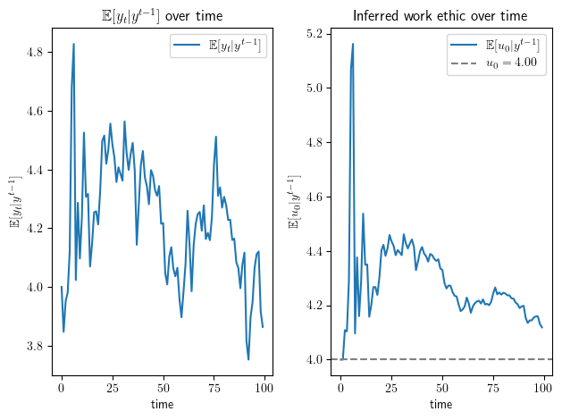
Fig. 46.1 Firm’s output forecast and inferred work ethic over time#
46.5. Some computational experiments#
Let’s look at \(\Sigma_0\) and \(\Sigma_{T-1}\) in order to see how much the firm learns about the hidden state during the horizon we have set.
print(Σ_t[:, :, 0])
[[4. 0.]
 [0. 4.]]
print(Σ_t[:, :, -1])
[[0.09403859 0.00997018]
 [0.00997018 0.01592704]]
Evidently, the conditional variances become smaller over time.
It is enlightening to portray how the firm’s conditional beliefs evolve by plotting contours of the conditional bivariate normal density of \(x_t\) given \(y^{t-1}\) at various \(t\)’s.
# Create a grid of points for contour plotting
h_range = np.linspace(x_hat_t[0, :].min()-0.5*Σ_t[0, 0, 1],
                      x_hat_t[0, :].max()+0.5*Σ_t[0, 0, 1], 100)
u_range = np.linspace(x_hat_t[1, :].min()-0.5*Σ_t[1, 1, 1],
                      x_hat_t[1, :].max()+0.5*Σ_t[1, 1, 1], 100)
h, u = np.meshgrid(h_range, u_range)

# Create a figure with subplots for each time step
fig, axs = plt.subplots(1, 3, figsize=(12, 7))

# Iterate through each time step
for i, t in enumerate(np.linspace(0, T-1, 3, dtype=int)):
    # Create a multivariate normal distribution with x_hat and Σ at time step t
    μ = x_hat_t[:, t]
    cov = Σ_t[:, :, t]
    mvn = multivariate_normal(mean=μ, cov=cov)

    # Evaluate the multivariate normal PDF on the grid
    pdf_values = mvn.pdf(np.dstack((h, u)))

    # Create a contour plot for the PDF
    con = axs[i].contour(h, u, pdf_values, cmap='viridis')
    axs[i].clabel(con, inline=1, fontsize=10)
    axs[i].set_title(f'Time Step {t}')
    axs[i].set_xlabel(r'$h_{{{}}}$'.format(str(t)))
    axs[i].set_ylabel(r'$u_{{{}}}$'.format(str(t)))

    cov_latex = (
        r'$\Sigma_{{{}}}= \begin{{bmatrix}} {:.2f} & {:.2f} \\ '
        r'{:.2f} & {:.2f} \end{{bmatrix}}$'
    ).format(t, cov[0, 0], cov[0, 1], cov[1, 0], cov[1, 1])
    axs[i].text(0.33, -0.15, cov_latex, transform=axs[i].transAxes)


plt.tight_layout()
plt.show()
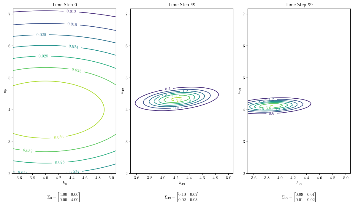
Fig. 46.2 Density contours for the firm’s belief about \(x_t\) at three dates#
Note how the accumulation of evidence \(y^{t-1}\) affects the shape of the density contours as sample size \(t\) grows.
Now let’s use our code to set the hidden state \(x_0\) to a particular vector in order to watch how a firm learns starting from some \(x_0\) we are interested in.
For example, let’s say \(h_0 = 0\) and \(u_0 = 4\).
Here is one way to do this.
# For example, we might want h_0 = 0 and u_0 = 4
μ_0 = np.array([[0.0],
                [4.0]])

# Create a LinearStateSpace object with Sigma_0 as a matrix of zeros
ss_example = LinearStateSpace(A, C, G, np.sqrt(R), mu_0=μ_0,
                              # This line forces exact h_0=0 and u_0=4
                              Sigma_0=np.zeros((2, 2))
                             )

T = 100
x, y = ss_example.simulate(T)
y = y.flatten()

# Now h_0=0 and u_0=4
h_0, u_0 = x[0, 0], x[1, 0]
print('h_0 =', h_0)
print('u_0 =', u_0)
h_0 = 0.0
u_0 = 4.0
Another way to accomplish the same goal is to use the following code.
# If we want to set the initial
# h_0 = hhat_0 = 0.0 and u_0 = uhat_0 = 4.0:
worker_example = create_worker(hhat_0=0.0, uhat_0=4.0)

# The firm's prior stays at the original xhat_0 and Σ_0
ss_example = LinearStateSpace(A, C, G, np.sqrt(R),
                              # This line takes h_0=hhat_0 and u_0=uhat_0
                              mu_0=worker_example.xhat_0,
                              # This line forces exact h_0=hhat_0 and u_0=uhat_0
                              Sigma_0=np.zeros((2, 2))
                             )

T = 100
x, y = ss_example.simulate(T)
y = y.flatten()

# Now h_0 and u_0 will be exactly hhat_0 and uhat_0
h_0, u_0 = x[0, 0], x[1, 0]
print('h_0 =', h_0)
print('u_0 =', u_0)
h_0 = 0.0
u_0 = 4.0
For this worker, let’s generate a plot like the one above.
# The firm filters output from ss_example using its prior beliefs
# xhat_0 and Σ_0
kalman = Kalman(ss_example, xhat_0, Σ_0)
Σ_t = []
y_hat_t = np.zeros(T)
u_hat_t = np.zeros(T)

# Then we iteratively update the Kalman filter class using
# observation y based on the linear state model above:
for t in range(T):
    # Record the firm's belief about x_t given y^{t-1}, before seeing y_t
    x_hat, Σ = kalman.x_hat, kalman.Sigma
    Σ_t.append(Σ)
    y_hat_t[t] = (G @ x_hat).item()
    u_hat_t[t] = x_hat[1].item()

    # Then incorporate the observation y_t and advance the filter to t+1
    kalman.update(y[t])


# Generate plots for y_hat_t and u_hat_t
fig, ax = plt.subplots(1, 2)

ax[0].plot(y_hat_t, label=r'$\mathbb{E}[y_t| y^{t-1}]$')
ax[0].set_xlabel('time')
ax[0].set_ylabel(r'$\mathbb{E}[y_t| y^{t-1}]$')
ax[0].set_title(r'$\mathbb{E}[y_t| y^{t-1}]$ over time')
ax[0].legend()

ax[1].plot(u_hat_t, label=r'$\mathbb{E}[u_0|y^{t-1}]$')
ax[1].axhline(y=u_0, color='grey',
            linestyle='dashed', label=fr'$u_0={u_0:.2f}$')
ax[1].set_xlabel('time')
ax[1].set_ylabel(r'$\mathbb{E}[u_0|y^{t-1}]$')
ax[1].set_title('Inferred work ethic over time')
ax[1].legend()

fig.tight_layout()
plt.show()
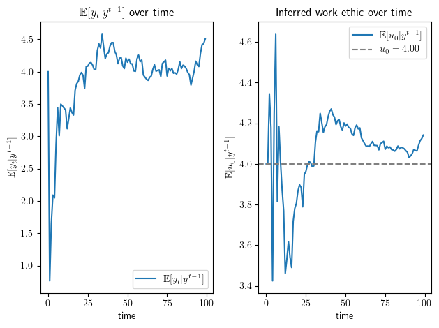
Fig. 46.3 Output forecast and inferred work ethic for the worker with \(u_0=4\)#
More generally, we can change some or all of the parameters defining a worker in our create_worker
namedtuple.
Here is an example.
# We can set these parameters when creating a worker -- just like classes!
hard_working_worker = create_worker(α=.4, β=.8,
                        hhat_0=7.0, uhat_0=100, σ_h=2.5, σ_u=3.2)

print(hard_working_worker)
WorkerModel(A=array([[0.4, 0.8],
       [0. , 1. ]]), C=array([[0.2],
       [0. ]]), G=array([1., 0.]), R=0.5, xhat_0=array([[  7.],
       [100.]]), Σ_0=array([[ 6.25,  0.  ],
       [ 0.  , 10.24]]))
We can also simulate the system for \(T = 100\) periods for different workers.
When effort feeds into output through human capital, so that \(g \neq 0\) and \(\beta \neq 0\), the firm’s uncertainty about \(u_0\) falls over time and the inferred work ethic converges toward the true \(u_0\).
If \(\beta = 0\), effort never affects \(h_t\), and if \(g = 0\), output carries no information about \(h_t\), so in either case the firm cannot learn \(u_0\) from output alone.
This shows that, under these observability conditions, the filter gradually teaches the firm about the worker’s effort.
For three workers, we first plot the gap between the firm’s inferred work ethic and the true \(u_0\) over time.
num_workers = 3
T = 100
fig, ax = plt.subplots(figsize=(7, 7))

for i in range(num_workers):
    worker = create_worker(uhat_0=4+2*i)
    simulate_workers(worker, T, ax, name=fr'$\hat u_0 = {4+2*i}$',
                     random_state=2 + i)
ax.set_ylim(ymin=-2, ymax=2)
ax.legend()
plt.show()
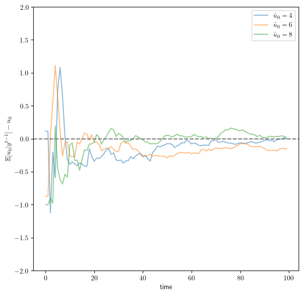
Fig. 46.4 Difference between inferred and true work ethic over time#
In this simulation the firm’s inferred work ethic moves toward the true \(u_0\).
Under the correctly specified observable linear-Gaussian model, the posterior mean of \(u_0\) is consistent, so this gap shrinks as the output history grows.
By setting diff=False, we instead plot the level of each worker’s inferred work ethic \(\mathbb{E}[u_0|y^{t-1}]\), shown together with a dashed line marking the true \(u_0\).
fig, ax = plt.subplots(figsize=(7, 7))

uhat_0s = [2, -2, 1]
αs = [0.2, 0.3, 0.5]
βs = [0.2, 0.9, 0.3]

for i, (uhat_0, α, β) in enumerate(zip(uhat_0s, αs, βs)):
    worker = create_worker(uhat_0=uhat_0, α=α, β=β)
    simulate_workers(worker, T, ax, diff=False,
                     name=r'$u_{{{}, 0}}$'.format(i),
                     random_state=3 + i)

ax.legend(bbox_to_anchor=(1, 0.5))
plt.show()
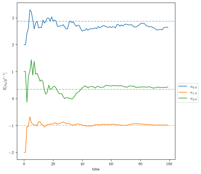
Fig. 46.5 Inferred work ethic over time for three workers#
These three workers differ in \(\alpha\) and \(\beta\) as well as in \(\hat u_0\), and the speed of learning differs sharply across them.
The worker with the largest \(\beta\), here \(u_{1,0}\) with \(\beta = 0.9\), settles onto its dashed true value almost immediately, while the worker with the smallest \(\beta\), here \(u_{0,0}\) with \(\beta = 0.2\), converges slower.
The reason is that effort affects output only through human capital, so in these stable examples with \(|\alpha| < 1\) its steady-state effect on output is governed by \(g \beta / (1 - \alpha)\), and a small \(\beta\) leaves the firm with too little signal to pin down \(u_0\) over this horizon.
The speed of learning also reflects the measurement noise \(R\), the shock scale \(c\), and the firm’s prior variances.
We can also give every worker the same true initial state, here \(h_0=2\) and \(u_0=1\), by passing a fixed μ_sim_0 and a zero Σ_sim_0 to simulate_workers.
fig, ax = plt.subplots(figsize=(7, 7))

μ_sim_0 = np.array([[2.0],
                    [1.0]])
Σ_sim_0 = np.zeros((2,2))

uhat_0s = [2, -2, 1]
αs = [0.2, 0.3, 0.5]
βs = [0.2, 0.9, 0.3]

for i, (uhat_0, α, β) in enumerate(zip(uhat_0s, αs, βs)):
    worker = create_worker(uhat_0=uhat_0, α=α, β=β)
    simulate_workers(worker, T, ax, μ_sim_0=μ_sim_0, Σ_sim_0=Σ_sim_0,
                     diff=False, name=r'$u_{{{}, 0}}$'.format(i))

# This controls the boundary of plots
ax.set_ylim(ymin=-3, ymax=3)
ax.legend(bbox_to_anchor=(1, 0.5))
plt.show()
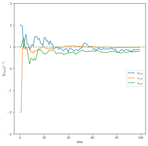
Fig. 46.6 Inferred work ethic when every worker starts at \(h_0=2\) and \(u_0=1\)#
Even though the firm begins from different prior means \(\hat u_0\), all three workers share the true work ethic \(u_0 = 1\), and the inferred paths converge to that common dashed line at speeds that again reflect each worker’s \(\beta\).
Finally, we track a single worker type under two different true effort levels, comparing a hard-working worker with \(u_0=100\) against a normal worker with \(u_0=30\).
T = 50
fig, ax = plt.subplots(figsize=(7, 7))

μ_sim_0_1 = np.array([[1],
                      [100]])
μ_sim_0_2 = np.array([[1],
                      [30]])
Σ_sim_0 = np.zeros((2, 2))

worker = create_worker(uhat_0=1, α=0.5, β=0.3)
simulate_workers(worker, T, ax, μ_sim_0=μ_sim_0_1, Σ_sim_0=Σ_sim_0,
                 diff=False, name=r'Hard-working worker')
simulate_workers(worker, T, ax, μ_sim_0=μ_sim_0_2, Σ_sim_0=Σ_sim_0,
                 diff=False, name=r'Normal worker')
ax.legend(bbox_to_anchor=(1, 0.5))
plt.show()
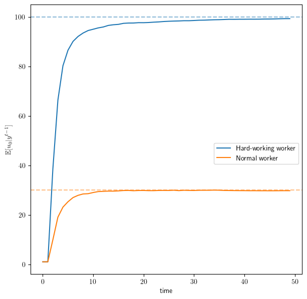
Fig. 46.7 A hard-working worker and a less hard-working worker#
Both inferred paths start from the firm’s common prior \(\hat u_0 = 1\) and climb toward their different true values, showing that the filter corrects the gap between prior and truth as evidence accumulates.
46.6. Future extensions#
We can do lots of enlightening experiments by creating new types of workers and letting the firm learn about their hidden (to the firm) states by observing just their output histories.