67. The Income Fluctuation Problem I: Discretization and VFI#
GPU
This lecture was built using a machine with access to a GPU — although it will also run without one.
Google Colab has a free tier with GPUs that you can access as follows:
Click on the “play” icon top right
Select Colab
Set the runtime environment to include a GPU
67.1. Overview#
In this lecture, we study an optimal savings problem for an infinitely lived consumer—the “common ancestor” described in [Ljungqvist and Sargent, 2018], section 1.3.
This savings problem is often called an income fluctuation problem or a household problem.
It is an essential sub-problem for many representative macroeconomic models
etc.
It is related to the decision problem in Optimal Savings III: Stochastic Returns but differs in significant ways.
For example,
The choice problem for the agent includes an additive income term that leads to an occasionally binding constraint.
Shocks affecting the budget constraint are correlated, forcing us to track an extra state variable.
We will begin by working with a relatively basic version of the model and solving it via old-fashioned discretization + value function iteration.
Although this approach is not the fastest or the most efficient, it is very robust and flexible.
For example, if we suddenly decided to add Epstein–Zin preferences, or modify ordinary conditional expectations to quantiles, the technique would continue to work well.
Note
The same is not true of some other methods we will deploy, such as the endogenous grid method.
This is a general rule of computation and analysis — while we can often come up with faster algorithms by exploiting structure, these new algorithms are typically less robust.
They are less robust precisely because they exploit more structure — which implies that they are, inevitably, more vulnerable to change.
In addition to Anaconda, this lecture will need the following libraries:
!pip install quantecon jax
We will use the following imports:
import quantecon as qe
import jax
import jax.numpy as jnp
import matplotlib.pyplot as plt
from typing import NamedTuple
from time import time
We’ll use 64 bit floats to gain extra precision.
jax.config.update("jax_enable_x64", True)
67.2. Set Up#
We study a household that chooses a state-contingent consumption plan \(\{c_t\}_{t \geq 0}\) to maximize
subject to
Here
\(c_t\) is consumption and \(c_t \geq 0\),
\(a_t\) is assets and \(a_t \geq 0\),
\(R = 1 + r\) is a gross rate of return, and
\((y_t)_{t \geq 0}\) is labor income, taking values in some finite set \(\mathsf Y\).
We assume below that labor income dynamics follow a discretized AR(1) process.
We set \(\mathsf S := \mathbb{R}_+ \times \mathsf Y\), which represents the state space.
The value function \(V \colon \mathsf S \to \mathbb{R}\) is defined by
where the maximization is over all feasible consumption sequences given \((a_0, y_0) = (a, y)\).
The Bellman equation is
where
In the code we use the function
the encapsulate the right hand side of the Bellman equation.
67.3. Code#
The following code defines a NamedTuple to store the model parameters and grids.
class Model(NamedTuple):
    β: float              # Discount factor
    R: float              # Gross interest rate
    γ: float              # CRRA parameter
    a_grid: jnp.ndarray   # Asset grid
    y_grid: jnp.ndarray   # Income grid
    Q: jnp.ndarray        # Markov matrix for income


def create_consumption_model(
        R=1.01,                    # Gross interest rate
        β=0.98,                    # Discount factor
        γ=2,                       # CRRA parameter
        a_min=0.01,                # Min assets
        a_max=10.0,                # Max assets
        a_size=150,                # Grid size
        ρ=0.9, ν=0.1, y_size=100   # Income parameters
    ):
    """
    Creates an instance of the consumption-savings model.

    """
    a_grid = jnp.linspace(a_min, a_max, a_size)
    mc = qe.tauchen(n=y_size, rho=ρ, sigma=ν)
    y_grid, Q = jnp.exp(mc.state_values), jax.device_put(mc.P)
    return Model(β, R, γ, a_grid, y_grid, Q)
Now we define the right hand side of the Bellman equation.
We’ll use a vectorized coding style reminiscent of Matlab and NumPy (avoiding all loops).
Your are invited to explore an alternative style based around jax.vmap in the Exercises.
@jax.jit
def B(v, model):
    """
    A vectorized version of the right-hand side of the Bellman equation
    (before maximization), which is a 3D array representing

        B(a, y, a′) = u(Ra + y - a′) + β Σ_y′ v(a′, y′) Q(y, y′)

    for all (a, y, a′).
    """

    # Unpack
    β, R, γ, a_grid, y_grid, Q = model
    a_size, y_size = len(a_grid), len(y_grid)

    # Compute current rewards r(a, y, ap) as array r[i, j, ip]
    a  = jnp.reshape(a_grid, (a_size, 1, 1))    # a[i]   ->  a[i, j, ip]
    y  = jnp.reshape(y_grid, (1, y_size, 1))    # z[j]   ->  z[i, j, ip]
    ap = jnp.reshape(a_grid, (1, 1, a_size))    # ap[ip] -> ap[i, j, ip]
    c = R * a + y - ap

    # Calculate continuation rewards at all combinations of (a, y, ap)
    v = jnp.reshape(v, (1, 1, a_size, y_size))  # v[ip, jp] -> v[i, j, ip, jp]
    Q = jnp.reshape(Q, (1, y_size, 1, y_size))  # Q[j, jp]  -> Q[i, j, ip, jp]
    EV = jnp.sum(v * Q, axis=3)                 # sum over last index jp

    # Compute the right-hand side of the Bellman equation
    return jnp.where(c > 0, c**(1-γ)/(1-γ) + β * EV, -jnp.inf)
Some readers might be concerned that we are creating high dimensional arrays, leading to inefficiency.
Could they be avoided by more careful vectorization?
In fact this is not necessary: this function will be JIT-compiled by JAX, and the JIT compiler will optimize compiled code to minimize memory use.
The Bellman operator \(T\) can be implemented by
@jax.jit
def T(v, model):
    "The Bellman operator."
    return jnp.max(B(v, model), axis=2)
The next function computes a \(v\)-greedy policy given \(v\) (i.e., the policy that maximizes the right-hand side of the Bellman equation.)
@jax.jit
def get_greedy(v, model):
    "Computes a v-greedy policy, returned as a set of indices."
    return jnp.argmax(B(v, model), axis=2)
67.3.1. Value function iteration#
Now we define a solver that implements VFI.
First we write a simple version using a standard Python loop.
def value_function_iteration_python(model, tol=1e-5, max_iter=10_000):
    """
    Implements VFI using successive approximation with a Python loop.
    """
    v = jnp.zeros((len(model.a_grid), len(model.y_grid)))
    error = tol + 1
    k = 0

    while error > tol and k < max_iter:
        v_new = T(v, model)
        error = jnp.max(jnp.abs(v_new - v))
        v = v_new
        k += 1

    return v, get_greedy(v, model)
Next we write a version that uses jax.lax.while_loop.
@jax.jit
def value_function_iteration(model, tol=1e-5, max_iter=10_000):
    """
    Implements VFI using successive approximation.
    """
    def body_fun(k_v_err):
        k, v, error = k_v_err
        v_new = T(v, model)
        error = jnp.max(jnp.abs(v_new - v))
        return k + 1, v_new, error

    def cond_fun(k_v_err):
        k, v, error = k_v_err
        return jnp.logical_and(error > tol, k < max_iter)

    v_init = jnp.zeros((len(model.a_grid), len(model.y_grid)))
    k, v_star, error = jax.lax.while_loop(cond_fun, body_fun,
                                          (1, v_init, tol + 1))
    return v_star, get_greedy(v_star, model)
67.3.2. Timing#
Let’s create an instance and compare the two implementations.
model = create_consumption_model()
First let’s time the Python version.
print("Starting VFI using Python loop.")
start = time()
v_star_python, σ_star_python = value_function_iteration_python(model)
python_time = time() - start
print(f"VFI completed in {python_time} seconds.")
Starting VFI using Python loop.
VFI completed in 2.578707218170166 seconds.
Now let’s time the jax.lax.while_loop version.
print("Starting VFI using jax.lax.while_loop.")
start = time()
v_star_jax, σ_star_jax = value_function_iteration(model)
v_star_jax.block_until_ready()
jax_with_compile = time() - start
print(f"VFI completed in {jax_with_compile} seconds.")
Starting VFI using jax.lax.while_loop.
VFI completed in 1.6127252578735352 seconds.
Let’s run it again to eliminate compile time.
start = time()
v_star_jax, σ_star_jax = value_function_iteration(model)
v_star_jax.block_until_ready()
jax_without_compile = time() - start
print(f"VFI completed in {jax_without_compile} seconds.")
VFI completed in 1.368882179260254 seconds.
Let’s check that the two implementations produce the same result.
print(f"Values match: {jnp.allclose(v_star_python, v_star_jax)}")
print(f"Policies match: {jnp.allclose(σ_star_python, σ_star_jax)}")
Values match: True
Policies match: True
Here’s the speedup from using jax.lax.while_loop.
print(f"Relative speed = {python_time / jax_without_compile:.2f}")
Relative speed = 1.88
67.3.3. Asset Dynamics#
To understand long-run behavior, let’s examine the asset accumulation dynamics under the optimal policy.
The following 45-degree diagram shows how assets evolve over time:
fig, ax = plt.subplots()

# Plot asset accumulation for first and last income states
for j, label in zip([0, -1], ['low income', 'high income']):
    # Get next-period assets for each current asset level
    a_next = model.a_grid[σ_star_jax[:, j]]
    ax.plot(model.a_grid, a_next, label=label)

# Add 45-degree line
ax.plot(model.a_grid, model.a_grid, 'k--', linewidth=0.5)
ax.set(xlabel='current assets', ylabel='next period assets')
ax.legend()
plt.show()
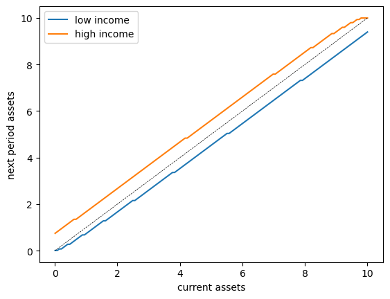
The plot shows the asset accumulation rule for each income state.
The dotted line is the 45-degree line, representing points where \(a_{t+1} = a_t\).
We see that:
For low income levels, assets tend to decrease (points below the 45-degree line)
For high income levels, assets tend to increase at low asset levels
The dynamics suggest convergence to a stationary distribution
67.4. Exercises#
Exercise 67.1
In this exercise, we explore an alternative approach to implementing value function iteration using jax.vmap.
For this simple optimal savings problem, direct vectorization is relatively easy.
In particular, it’s straightforward to express the right hand side of the Bellman equation as an array that stores evaluations of the function at every state and control.
However, for more complex models, direct vectorization can be much harder.
For this reason, it helps to have another approach to fast JAX implementations up our sleeves.
Your task is to implement a version that:
writes the right hand side of the Bellman operator as a function of individual states and controls, and
applies
jax.vmapon the outside to achieve a parallelized solution.
Specifically:
Rewrite
Bto take indices(i, j, ip)corresponding to(a, y, a′)and compute the Bellman equation for those specific indices.Use
jax.vmapsuccessively to vectorize over all indices (use staged vmap as shown in earlier examples).Implement
T_vmapandget_greedy_vmapfunctions using the vectorizedB.Implement
value_iteration_vmapusingjax.lax.while_loop.Test that your implementation produces the same results as the direct vectorization approach.
Compare the execution times of both approaches.
Solution
Here’s one solution.
First let’s rewrite B to work with individual indices:
def B(v, model, i, j, ip):
    """
    The right-hand side of the Bellman equation before maximization, which takes
    the form

        B(a, y, a′) = u(Ra + y - a′) + β Σ_y′ v(a′, y′) Q(y, y′)

    The indices are (i, j, ip) -> (a, y, a′).
    """
    β, R, γ, a_grid, y_grid, Q = model
    a, y, ap  = a_grid[i], y_grid[j], a_grid[ip]
    c = R * a + y - ap
    EV = jnp.sum(v[ip, :] * Q[j, :])
    return jnp.where(c > 0, c**(1-γ)/(1-γ) + β * EV, -jnp.inf)
Now we successively apply vmap to simulate nested loops.
B_1    = jax.vmap(B,   in_axes=(None, None, None, None, 0))
B_2    = jax.vmap(B_1, in_axes=(None, None, None, 0,    None))
B_vmap = jax.vmap(B_2, in_axes=(None, None, 0,    None, None))
Here’s the Bellman operator and the get_greedy functions for the vmap case.
@jax.jit
def T_vmap(v, model):
    "The Bellman operator."
    a_indices = jnp.arange(len(model.a_grid))
    y_indices = jnp.arange(len(model.y_grid))
    B_values = B_vmap(v, model, a_indices, y_indices, a_indices)
    return jnp.max(B_values, axis=-1)

@jax.jit
def get_greedy_vmap(v, model):
    "Computes a v-greedy policy, returned as a set of indices."
    a_indices = jnp.arange(len(model.a_grid))
    y_indices = jnp.arange(len(model.y_grid))
    B_values = B_vmap(v, model, a_indices, y_indices, a_indices)
    return jnp.argmax(B_values, axis=-1)
Here’s the iteration routine.
def value_iteration_vmap(model, tol=1e-5, max_iter=10_000):
    """
    Implements VFI using vmap and successive approximation.
    """
    def body_fun(k_v_err):
        k, v, error = k_v_err
        v_new = T_vmap(v, model)
        error = jnp.max(jnp.abs(v_new - v))
        return k + 1, v_new, error

    def cond_fun(k_v_err):
        k, v, error = k_v_err
        return jnp.logical_and(error > tol, k < max_iter)

    v_init = jnp.zeros((len(model.a_grid), len(model.y_grid)))
    k, v_star, error = jax.lax.while_loop(cond_fun, body_fun,
                                          (1, v_init, tol + 1))
    return v_star, get_greedy_vmap(v_star, model)
Let’s see how long it takes to solve the model using the vmap method.
print("Starting VFI using vmap.")
start = time()
v_star_vmap, σ_star_vmap = value_iteration_vmap(model)
v_star_vmap.block_until_ready()
jax_vmap_with_compile = time() - start
print(f"VFI completed in {jax_vmap_with_compile} seconds.")
Starting VFI using vmap.
VFI completed in 0.6073920726776123 seconds.
Let’s run it again to get rid of compile time.
start = time()
v_star_vmap, σ_star_vmap = value_iteration_vmap(model)
v_star_vmap.block_until_ready()
jax_vmap_without_compile = time() - start
print(f"VFI completed in {jax_vmap_without_compile} seconds.")
VFI completed in 0.3697941303253174 seconds.
We need to make sure that we got the same result.
print(jnp.allclose(v_star_vmap, v_star_jax))
print(jnp.allclose(σ_star_vmap, σ_star_jax))
True
True
Here’s the comparison with the first JAX implementation (which used direct vectorization).
print(f"Relative speed = {jax_without_compile / jax_vmap_without_compile}")
Relative speed = 3.7017412311439695
The execution times for the two JAX versions are relatively similar.
However, as emphasized above, having a second method up our sleeves (i.e, the
vmap approach) will be helpful when confronting dynamic programs with more
sophisticated Bellman equations.