90. Transitions in an Overlapping Generations Model#
In addition to what’s in Anaconda, this lecture will need the following libraries:
!pip install --upgrade quantecon
90.1. Introduction#
This lecture presents a life-cycle model consisting of overlapping generations of two-period lived people proposed by Peter Diamond [Diamond, 1965].
We’ll present the version that was analyzed in chapter 2 of Auerbach and Kotlikoff (1987) [Auerbach and Kotlikoff, 1987].
Auerbach and Kotlikoff (1987) used their two period model as a warm-up for their analysis of overlapping generation models of long-lived people that is the main topic of their book.
Their model of two-period lived overlapping generations is a useful starting point because
it sets forth the structure of interactions between generations of different agents who are alive at a given date
it activates forces and tradeoffs confronting the government and successive generations of people
it is good laboratory for studying connections between government tax and subsidy programs and for policies for issuing and servicing government debt
some interesting experiments involving transitions from one steady state to another can be computed by hand
it is a good setting for illustrating a shooting method for solving a system of non-linear difference equations with initial and terminal condition
Note
Auerbach and Kotlikoff use computer code to calculate transition paths for their models with long-lived people.
We take the liberty of extending Auerbach and Kotlikoff’s chapter 2 model to study some arrangements for redistributing resources across generations
these take the form of a sequence of age-specific lump sum taxes and transfers
We study how these arrangements affect capital accumulation and government debt
90.2. Setting#
Time is discrete and is indexed by \(t=0, 1, 2, \ldots\).
The economy lives forever, but the people inside it do not.
At each time \( t \geq 0\) a representative old person and a representative young person are alive.
At time \(t\) a representative old person coexists with a representative young person who will become an old person at time \(t+1\).
We assume that the population size is constant over time.
A young person works, saves, and consumes.
An old person dissaves and consumes, but does not work,
A government lives forever, i.e., at \(t=0, 1, 2, \ldots \).
Each period \(t \geq 0\), the government taxes, spends, transfers, and borrows.
Initial conditions set outside the model at time \(t=0\) are
\(K_0\) – initial capital stock brought into time \(t=0\) by a representative initial old person
\(D_0\) – government debt falling due at \(t=0\) and owned by a representative old person at time \(t=0\)
\(K_0\) and \(D_0\) are both measured in units of time \(0\) goods.
A government policy consists of five sequences \(\{G_t, D_t, \tau_t, \delta_{ot}, \delta_{yt}\}_{t=0}^\infty \) whose components are
\(\tau_t\) – flat rate tax at time \(t\) on wages and earnings from capital and government bonds
\(D_t\) – one-period government bond principal due at time \(t\), per capita
\(G_t\) – government purchases of goods at time \(t\), per capita
\(\delta_{yt}\) – a lump sum tax on each young person at time \(t\)
\(\delta_{ot}\) – a lump sum tax on each old person at time \(t\)
An allocation is a collection of sequences \(\{C_{yt}, C_{ot}, K_{t+1}, L_t, Y_t, G_t\}_{t=0}^\infty \); constituents of the sequences include
\(K_t\) – physical capital per capita
\(L_t\) – labor per capita
\(Y_t\) – output per capita
and also
\(C_{yt}\) – consumption of young person at time \(t \geq 0\)
\(C_{ot}\) – consumption of old person at time \(t \geq 0\)
\(K_{t+1} - K_t \equiv I_t \) – investment in physical capital at time \(t \geq 0\)
\(G_t\) – government purchases
National income and product accounts consist of a sequence of equalities
\(Y_t = C_{yt} + C_{ot} + (K_{t+1} - K_t) + G_t, \quad t \geq 0\)
A price system is a pair of sequences \(\{W_t, r_t\}_{t=0}^\infty\); constituents of a price sequence include rental rates for the factors of production
\(W_t\) – rental rate for labor at time \(t \geq 0\)
\(r_t\) – rental rate for capital at time \(t \geq 0\)
90.3. Production#
There are two factors of production, physical capital \(K_t\) and labor \(L_t\).
Capital does not depreciate.
The initial capital stock \(K_0\) is owned by the representative initial old person, who rents it to the firm at time \(0\).
Net investment rate \(I_t\) at time \(t\) is
The capital stock at time \(t\) emerges from cumulating past rates of investment:
A Cobb-Douglas technology converts physical capital \(K_t\) and labor services \(L_t\) into output \(Y_t\)
90.4. Government#
At time \(t-1\), the government issues one-period risk-free debt that promises to pay \(D_t\) time \(t\) goods per capita at time \(t\).
Young people at time \(t\) purchase government debt \(D_{t+1}\) that matures at time \(t+1\).
Government debt issued at \(t\) bears a before-tax net rate of interest rate of \(r_{t}\) at time \(t+1\).
The government budget constraint at time \(t \geq 0\) is
or
Total tax collections net of transfers equal \(T_t\) and satisfy
90.5. Activities in Factor Markets#
Old people: At each \(t \geq 0\), a representative old person
brings \(K_t\) and \(D_t\) into the period,
rents capital to a representative firm for \(r_{t} K_t\),
pays taxes \(\tau_t r_t (K_t+ D_t)\) on its rental and interest earnings,
pays a lump sum tax \(\delta_{ot}\) to the government,
sells \(K_t\) to a young person.
Young people: At each \(t \geq 0\), a representative young person
sells one unit of labor services to a representative firm for \(W_t\) in wages,
pays taxes \(\tau_t W_t\) on its labor earnings
pays a lump sum tax \(\delta_{yt}\) to the goverment,
spends \(C_{yt}\) on consumption,
acquires non-negative assets \(A_{t+1}\) consisting of a sum of physical capital \(K_{t+1}\) and one-period government bonds \(D_{t+1}\) that mature at \(t+1\).
Note
If a lump-sum tax is negative, it means that the government pays the person a subsidy.
90.6. Representative firm’s problem#
The representative firm hires labor services from young people at competitive wage rate \(W_t\) and hires capital from old people at competitive rental rate \(r_t\).
The rental rate on capital \(r_t\) equals the interest rate on government one-period bonds.
Units of the rental rates are:
for \(W_t\), output at time \(t\) per unit of labor at time \(t\)
for \(r_t\), output at time \(t\) per unit of capital at time \(t\)
We take output at time \(t\) as numeraire, so the price of output at time \(t\) is one.
The firm’s profits at time \(t\) are
To maximize profits a firm equates marginal products to rental rates:
Output can be consumed either by old people or young people; or sold to young people who use it to augment the capital stock; or sold to the government for uses that do not generate utility for the people in the model (i.e., “it is thrown into the ocean”).
The firm thus sells output to old people, young people, and the government.
90.7. Individuals’ problems#
90.7.1. Initial old person#
At time \(t=0\), a representative initial old person is endowed with \((1 + r_0(1 - \tau_0)) A_0\) in initial assets.
It must pay a lump sum tax to (if positive) or receive a subsidy from (if negative) \(\delta_{ot}\) the government.
An old person’s budget constraint is
An initial old person’s utility function is \(C_{o0}\), so the person’s optimal consumption plan is provided by equation (90.4).
90.7.2. Young person#
At each \(t \geq 0\), a young person inelastically supplies one unit of labor and in return receives pre-tax labor earnings of \(W_t\) units of output.
A young person’s post-tax-and-transfer earnings are \(W_t (1 - \tau_t) - \delta_{yt}\).
At each \(t \geq 0\), a young person chooses a consumption plan \(C_{yt}, C_{ot+1}\) to maximize the Cobb-Douglas utility function
subject to the following budget constraints at times \(t\) and \(t+1\):
Solving the second equation of (90.6) for savings \(A_{t+1}\) and substituting it into the first equation implies the present value budget constraint
To solve the young person’s choice problem, form a Lagrangian
where \(\lambda\) is a Lagrange multiplier on the intertemporal budget constraint (90.7).
After several lines of algebra, the intertemporal budget constraint (90.7) and the first-order conditions for maximizing \({\mathcal L}\) with respect to \(C_{yt}, C_{ot+1}\) imply that an optimal consumption plan satisfies
The first-order condition for minimizing Lagrangian (90.8) with respect to the Lagrange multipler \(\lambda\) recovers the budget constraint (90.7), which, using (90.9) gives the optimal savings plan
90.8. Equilbrium#
Definition: An equilibrium is an allocation, a government policy, and a price system with the properties that
given the price system and the government policy, the allocation solves
representative firms’ problems for \(t \geq 0\)
individual persons’ problems for \(t \geq 0\)
given the price system and the allocation, the government budget constraint is satisfied for all \(t \geq 0\).
90.9. Next steps#
To begin our analysis of equilibrium outcomes, we’ll study the special case of the model with which Auerbach and Kotlikoff (1987) [Auerbach and Kotlikoff, 1987] began their analysis in chapter 2.
It can be solved by hand.
We shall do that next.
After we derive a closed form solution, we’ll pretend that we don’t know and will compute equilibrium outcome paths.
We’ll do that by first formulating an equilibrium as a fixed point of a mapping from sequences of factor prices and tax rates to sequences of factor prices and tax rates.
We’ll compute an equilibrium by iterating to convergence on that mapping.
90.10. Closed form solution#
To get the special chapter 2 case of Auerbach and Kotlikoff (1987) [Auerbach and Kotlikoff, 1987], we set both \(\delta_{ot}\) and \(\delta_{yt}\) to zero.
As our special case of (90.9), we compute the following consumption-savings plan for a representative young person:
Using (90.3) and \(A_t = K_t + D_t\), we obtain the following closed form transition law for capital:
90.10.1. Steady states#
From (90.11) and the government budget constraint (90.2), we compute time-invariant or steady state values \(\hat K, \hat D, \hat T\):
These imply
Let’s take an example in which
there is no initial government debt, \(D_t=0\),
government consumption \(G_t\) equals \(15\%\) of output \(Y_t\)
Our formulas for steady-state values tell us that
90.10.2. Implementation#
import numpy as np
import matplotlib.pyplot as plt
from numba import jit
from quantecon.optimize import brent_max
For parameters \(\alpha = 0.3\) and \(\beta = 0.5\), let’s compute \(\hat{K}\):
# parameters
α = 0.3
β = 0.5

# steady states of τ and D
τ_hat = 0.15
D_hat = 0.

# solve for steady state of K
K_hat = ((1 - τ_hat) * (1 - α) * (1 - β)) ** (1 / (1 - α))
K_hat
0.17694509514972878
Knowing \(\hat K\), we can calculate other equilibrium objects.
Let’s first define some Python helper functions.
@jit
def K_to_Y(K, α):

    return K ** α

@jit
def K_to_r(K, α):

    return α * K ** (α - 1)

@jit
def K_to_W(K, α):

    return (1 - α) * K ** α

@jit
def K_to_C(K, D, τ, r, α, β):

    # optimal consumption for the old when δ=0
    A = K + D
    Co = A * (1 + r * (1 - τ))

    # optimal consumption for the young when δ=0
    W = K_to_W(K, α)
    Cy = β * W * (1 - τ)

    return Cy, Co
We can use these helper functions to obtain steady state values \(\hat{Y}\), \(\hat{r}\), and \(\hat{W}\) associated with steady state values \(\hat{K}\) and \(\hat{r}\).
Y_hat, r_hat, W_hat = K_to_Y(K_hat, α), K_to_r(K_hat, α), K_to_W(K_hat, α)
Y_hat, r_hat, W_hat
(0.5947734290747186, 1.0084033613445376, 0.41634140035230305)
Since steady state government debt \(\hat{D}\) is \(0\), all taxes are used to pay for government expenditures
G_hat = τ_hat * Y_hat
G_hat
0.0892160143612078
We use the optimal consumption plans to find steady state consumptions for young and old
Cy_hat, Co_hat = K_to_C(K_hat, D_hat, τ_hat, r_hat, α, β)
Cy_hat, Co_hat
(0.17694509514972878, 0.32861231956378195)
Let’s store the steady state quantities and prices using an array called init_ss
init_ss = np.array([K_hat, Y_hat, Cy_hat, Co_hat,     # quantities
                    W_hat, r_hat,                     # prices
                    τ_hat, D_hat, G_hat               # policies
                    ])
90.10.3. Transitions#
We have computed a steady state in which the government policy sequences are each constant over time.
We’ll use this steady state as an initial condition at time \(t=0\) for another economy in which government policy sequences are with time-varying sequences.
To make sense of our calculation, we’ll treat \(t=0\) as time when a huge unanticipated shock occurs in the form of
a time-varying government policy sequences that disrupts an original steady state
new government policy sequences are eventually time-invariant in the sense that after some date \(T >0\), each sequence is constant over time.
sudden revelation of a new government policy in the form of sequences starting at time \(t=0\)
We assume that everyone, including old people at time \(t=0\), knows the new government policy sequence and chooses accordingly.
As the capital stock and other aggregates adjust to the fiscal policy change over time, the economy will approach a new steady state.
We can find a transition path from an old steady state to a new steady state by employing a fixed-point algorithm in a space of sequences.
But in our special case with its closed form solution, we have available a simpler and faster approach.
Here we define a Python class ClosedFormTrans that computes length \(T\) transition path in response to a particular fiscal policy change.
We choose \(T\) large enough so that we have gotten very close to a new steady state after \(T\) periods.
The class takes three keyword arguments, τ_pol, D_pol, and G_pol.
These are sequences of tax rate, government debt level, and government purchases, respectively.
In each policy experiment below, we will pass two out of three as inputs required to depict a fiscal policy.
We’ll then compute the single remaining undetermined policy variable from the government budget constraint.
When we simulate transition paths, it is useful to distinguish state variables at time \(t\) such as \(K_t, Y_t, D_t, W_t, r_t\) from control variables that include \(C_{yt}, C_{ot}, \tau_{t}, G_t\).
class ClosedFormTrans:
    """
    This class simulates length T transitional path of a economy
    in response to a fiscal policy change given its initial steady
    state. The simulation is based on the closed form solution when
    the lump sum taxations are absent.

    """

    def __init__(self, α, β):

        self.α, self.β = α, β

    def simulate(self,
                T,           # length of transitional path to simulate
                init_ss,     # initial steady state
                τ_pol=None,  # sequence of tax rates
                D_pol=None,  # sequence of government debt levels
                G_pol=None): # sequence of government purchases

        α, β = self.α, self.β

        # unpack the steady state variables
        K_hat, Y_hat, Cy_hat, Co_hat = init_ss[:4]
        W_hat, r_hat = init_ss[4:6]
        τ_hat, D_hat, G_hat = init_ss[6:9]

        # initialize array containers
        # K, Y, Cy, Co
        quant_seq = np.empty((T+1, 4))

        # W, r
        price_seq = np.empty((T+1, 2))

        # τ, D, G
        policy_seq = np.empty((T+2, 3))

        # t=0, starting from steady state
        K0, Y0 = K_hat, Y_hat
        W0, r0 = W_hat, r_hat
        D0 = D_hat

        # fiscal policy
        if τ_pol is None:
            D1 = D_pol[1]
            G0 = G_pol[0]
            τ0 = (G0 + (1 + r0) * D0 - D1) / (Y0 + r0 * D0)
        elif D_pol is None:
            τ0 = τ_pol[0]
            G0 = G_pol[0]
            D1 = (1 + r0) * D0 + G0 - τ0 * (Y0 + r0 * D0)
        elif G_pol is None:
            D1 = D_pol[1]
            τ0 = τ_pol[0]
            G0 = τ0 * (Y0 + r0 * D0) + D1 - (1 + r0) * D0

        # optimal consumption plans
        Cy0, Co0 = K_to_C(K0, D0, τ0, r0, α, β)

        # t=0 economy
        quant_seq[0, :] = K0, Y0, Cy0, Co0
        price_seq[0, :] = W0, r0
        policy_seq[0, :] = τ0, D0, G0
        policy_seq[1, 1] = D1

        # starting from t=1 to T
        for t in range(1, T+1):

            # transition of K
            K_old, τ_old = quant_seq[t-1, 0], policy_seq[t-1, 0]
            D = policy_seq[t, 1]
            K = K_old ** α * (1 - τ_old) * (1 - α) * (1 - β) - D

            # output, capital return, wage
            Y, r, W = K_to_Y(K, α), K_to_r(K, α), K_to_W(K, α)

            # to satisfy the government budget constraint
            if τ_pol is None:
                D = D_pol[t]
                D_next = D_pol[t+1]
                G = G_pol[t]
                τ = (G + (1 + r) * D - D_next) / (Y + r * D)
            elif D_pol is None:
                τ = τ_pol[t]
                G = G_pol[t]
                D = policy_seq[t, 1]
                D_next = (1 + r) * D + G - τ * (Y + r * D)
            elif G_pol is None:
                D = D_pol[t]
                D_next = D_pol[t+1]
                τ = τ_pol[t]
                G = τ * (Y + r * D) + D_next - (1 + r) * D

            # optimal consumption plans
            Cy, Co = K_to_C(K, D, τ, r, α, β)

            # store time t economy aggregates
            quant_seq[t, :] = K, Y, Cy, Co
            price_seq[t, :] = W, r
            policy_seq[t, 0] = τ
            policy_seq[t+1, 1] = D_next
            policy_seq[t, 2] = G

        self.quant_seq = quant_seq
        self.price_seq = price_seq
        self.policy_seq = policy_seq

        return quant_seq, price_seq, policy_seq

    def plot(self):

        quant_seq = self.quant_seq
        price_seq = self.price_seq
        policy_seq = self.policy_seq

        fig, axs = plt.subplots(3, 3, figsize=(14, 10))

        # quantities
        for i, name in enumerate(['K', 'Y', 'Cy', 'Co']):
            ax = axs[i//3, i%3]
            ax.plot(range(T+1), quant_seq[:T+1, i], label=name)
            ax.hlines(init_ss[i], 0, T+1, color='r', linestyle='--')
            ax.legend()
            ax.set_xlabel('t')

        # prices
        for i, name in enumerate(['W', 'r']):
            ax = axs[(i+4)//3, (i+4)%3]
            ax.plot(range(T+1), price_seq[:T+1, i], label=name)
            ax.hlines(init_ss[i+4], 0, T+1, color='r', linestyle='--')
            ax.legend()
            ax.set_xlabel('t')

        # policies
        for i, name in enumerate(['τ', 'D', 'G']):
            ax = axs[(i+6)//3, (i+6)%3]
            ax.plot(range(T+1), policy_seq[:T+1, i], label=name)
            ax.hlines(init_ss[i+6], 0, T+1, color='r', linestyle='--')
            ax.legend()
            ax.set_xlabel('t')
We can create an instance closed for model parameters \(\{\alpha, \beta\}\) and use it for various fiscal policy experiments.
closed = ClosedFormTrans(α, β)
90.10.4. Experiment 1: Tax cut#
To illustrate the power of ClosedFormTrans, let’s first experiment with the following fiscal policy change:
at \(t=0\), the government unexpectedly announces a one-period tax cut, \(\tau_0 =(1-\frac{1}{3}) \hat{\tau}\), by issuing government debt \(\bar{D}\)
from \(t=1\), the government will keep \(D_t=\bar{D}\) and adjust \(\tau_{t}\) to collect taxation to pay for the government consumption and interest payments on the debt
government consumption \(G_t\) will be fixed at \(0.15 \hat{Y}\)
The following equations completely characterize the equilibrium transition path originating from the initial steady state
We can simulate the transition for \(20\) periods, after which the economy will be close to a new steady state.
The first step is to prepare sequences of policy variables that describe fiscal policy.
We must define sequences of government expenditure \(\{G_t\}_{t=0}^{T}\) and debt level \(\{D_t\}_{t=0}^{T+1}\) in advance, then pass them to the solver.
T = 20

# tax cut
τ0 = τ_hat * (1 - 1/3)

# sequence of government purchase
G_seq = τ_hat * Y_hat * np.ones(T+1)

# sequence of government debt
D_bar = G_hat - τ0 * Y_hat
D_seq = np.ones(T+2) * D_bar
D_seq[0] = D_hat
Let’s use the simulate method of closed to compute dynamic transitions.
Note that we leave τ_pol as None, since the tax rates need to be determined to satisfy the government budget constraint.
quant_seq1, price_seq1, policy_seq1 = closed.simulate(T, init_ss,
                                                      D_pol=D_seq,
                                                      G_pol=G_seq)
closed.plot()

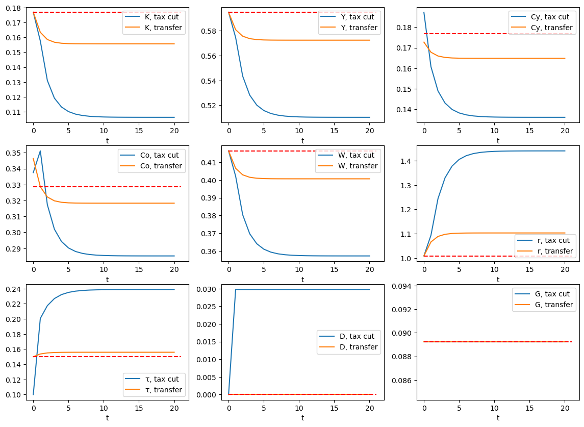
We can also experiment with a lower tax cut rate, such as \(0.2\).
# lower tax cut rate
τ0 = 0.15 * (1 - 0.2)

# the corresponding debt sequence
D_bar = G_hat - τ0 * Y_hat
D_seq = np.ones(T+2) * D_bar
D_seq[0] = D_hat

quant_seq2, price_seq2, policy_seq2 = closed.simulate(T, init_ss,
                                                      D_pol=D_seq,
                                                      G_pol=G_seq)
fig, axs = plt.subplots(3, 3, figsize=(14, 10))

# quantities
for i, name in enumerate(['K', 'Y', 'Cy', 'Co']):
    ax = axs[i//3, i%3]
    ax.plot(range(T+1), quant_seq1[:T+1, i], label=f'{name}, 1/3')
    ax.plot(range(T+1), quant_seq2[:T+1, i], label=f'{name}, 0.2')
    ax.hlines(init_ss[i], 0, T+1, color='r', linestyle='--')
    ax.legend()
    ax.set_xlabel('t')

# prices
for i, name in enumerate(['W', 'r']):
    ax = axs[(i+4)//3, (i+4)%3]
    ax.plot(range(T+1), price_seq1[:T+1, i], label=f'{name}, 1/3')
    ax.plot(range(T+1), price_seq2[:T+1, i], label=f'{name}, 0.2')
    ax.hlines(init_ss[i+4], 0, T+1, color='r', linestyle='--')
    ax.legend()
    ax.set_xlabel('t')

# policies
for i, name in enumerate(['τ', 'D', 'G']):
    ax = axs[(i+6)//3, (i+6)%3]
    ax.plot(range(T+1), policy_seq1[:T+1, i], label=f'{name}, 1/3')
    ax.plot(range(T+1), policy_seq2[:T+1, i], label=f'{name}, 0.2')
    ax.hlines(init_ss[i+6], 0, T+1, color='r', linestyle='--')
    ax.legend()
    ax.set_xlabel('t')
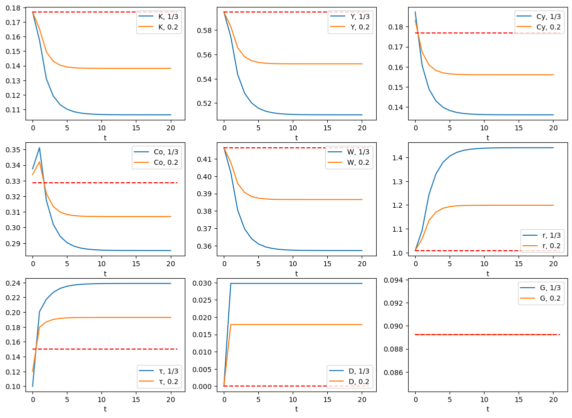
The economy with lower tax cut rate at \(t=0\) has the same transitional pattern, but is less distorted, and it converges to a new steady state with higher physical capital stock.
90.10.5. Experiment 2: Government asset accumulation#
Assume that the economy is initially in the same steady state.
Now the government promises to cut its spending on services and goods by half \(\forall t \geq 0\).
The government targets the same tax rate \(\tau_t=\hat{\tau}\) and to accumulate assets \(-D_t\) over time.
To conduct this experiment, we pass τ_seq and G_seq as inputs and let D_pol be determined along the path by satisfying the government budget constraint.
# government expenditure cut by a half
G_seq = τ_hat * 0.5 * Y_hat * np.ones(T+1)

# targeted tax rate
τ_seq = τ_hat * np.ones(T+1)

closed.simulate(T, init_ss, τ_pol=τ_seq, G_pol=G_seq);
closed.plot()
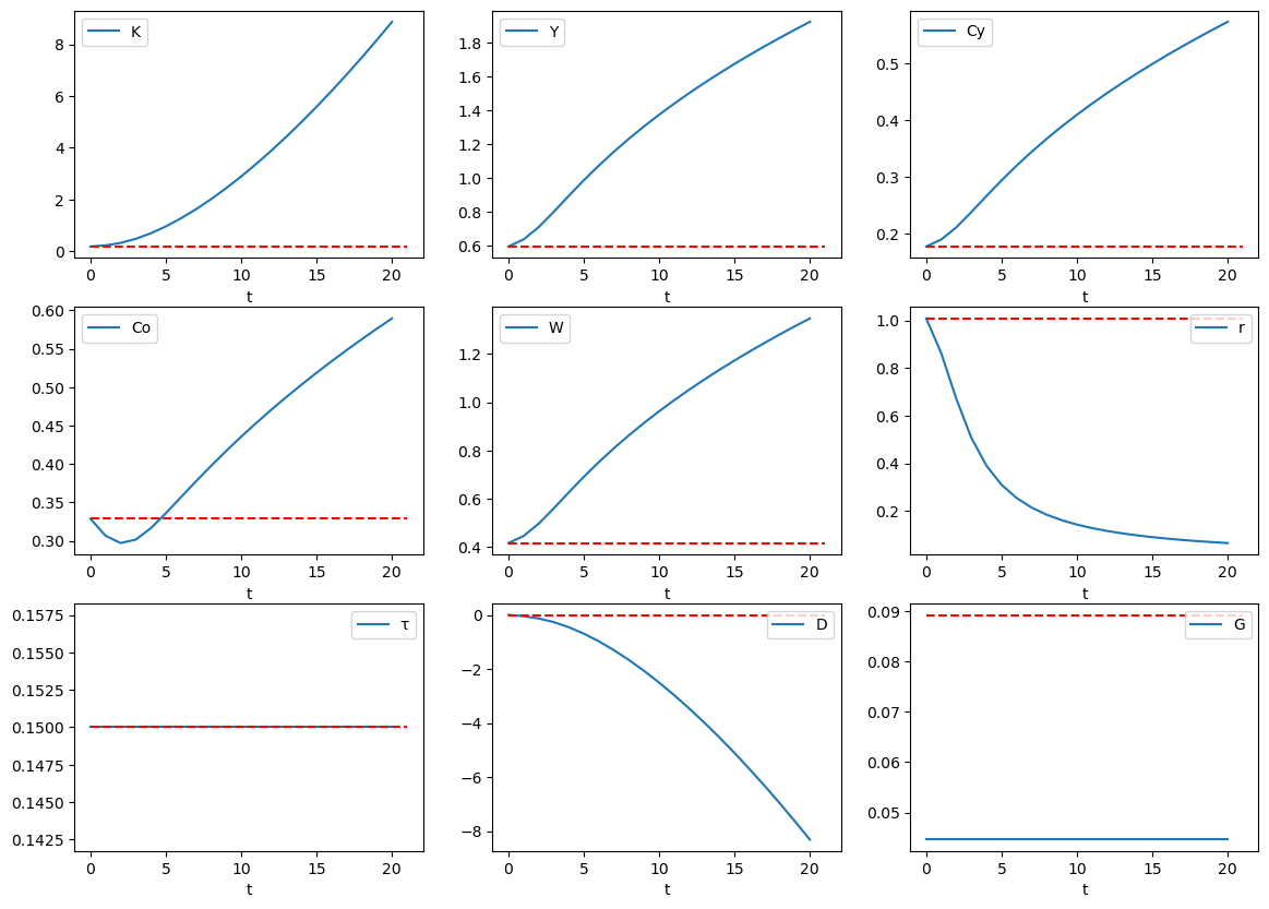
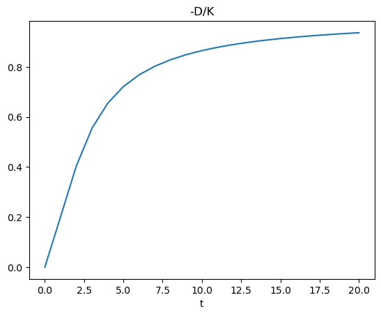
As the government accumulates the asset and uses it in production, the rental rate on capital falls and private investment falls.
As a result, the ratio \(-\frac{D_t}{K_t}\) of the government asset to physical capital used in production will increase over time
plt.plot(range(T+1), -closed.policy_seq[:-1, 1] / closed.quant_seq[:, 0])
plt.xlabel('t')
plt.title('-D/K');
We want to know how this policy experiment affects individuals.
In the long run, future cohorts will enjoy higher consumption throughout their lives because they will earn higher labor income when they work.
However, in the short run, old people suffer because increases in their labor income are not big enough to offset their losses of capital income.
Such distinct long run and short run effects motivate us to study transition paths.
Note
Although the consumptions in the new steady state are strictly higher, it is at a cost of fewer public services and goods.
90.10.6. Experiment 3: Temporary expenditure cut#
Let’s now investigate a scenario in which the government also cuts its spending by half and accumulates the asset.
But now let the government cut its expenditures only at \(t=0\).
From \(t \geq 1\), the government expeditures return to \(\hat{G}\) and \(\tau_t\) adjusts to maintain the asset level \(-D_t = -D_1\).
# sequence of government purchase
G_seq = τ_hat * Y_hat * np.ones(T+1)
G_seq[0] = 0

# sequence of government debt
D_bar = G_seq[0] - τ_hat * Y_hat
D_seq = D_bar * np.ones(T+2)
D_seq[0] = D_hat

closed.simulate(T, init_ss, D_pol=D_seq, G_pol=G_seq);
closed.plot()
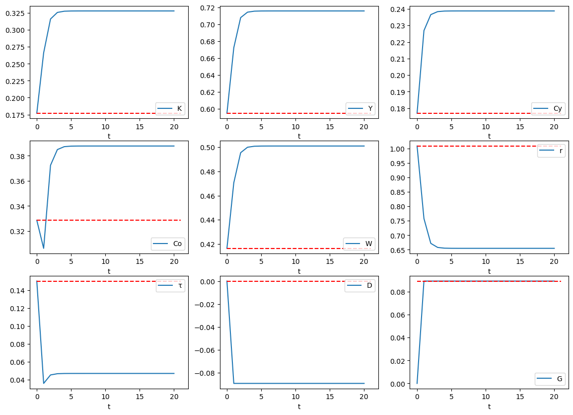
The economy quickly converges to a new steady state with higher physical capital stock, lower interest rate, higher wage rate, and higher consumptions for both the young and the old.
Even though government expenditure \(G_t\) returns to its high initial level from \(t \geq 1\), the government can balance the budget at a lower tax rate because it gathers additional revenue \(-r_t D_t\) from the asset accumulated during the temporary cut in the spendings.
As in Experiment 2: Government asset accumulation, old perople early in the transition periods suffer from this policy shock.
90.11. A computational strategy#
With the preceding caluations, we studied dynamic transitions instigated by alternative fiscal policies.
In all these experiments, we maintained the assumption that lump sum taxes were absent so that \(\delta_{yt}=0, \delta_{ot}=0\).
In this section, we investigate the transition dynamics when the lump sum taxes are present.
The government will use lump sum taxes and transfers to redistribute resources across successive generations.
Including lump sum taxes disrupts closed form solution because of how they make optimal consumption and saving plans depend on future prices and tax rates.
Therefore, we compute equilibrium transitional paths by finding a fixed point of a mapping from sequences to sequences.
that fixed point pins down an equilibrium
To set the stage for the entry of the mapping whose fixed point we seek, we return to concepts introduced in section Equilbrium.
Definition: Given parameters \(\{\alpha\), \(\beta\}\), a competitive equilibrium consists of
sequences of optimal consumptions \(\{C_{yt}, C_{ot}\}\)
sequences of prices \(\{W_t, r_t\}\)
sequences of capital stock and output \(\{K_t, Y_t\}\)
sequences of tax rates, government assets (debt), government purchases \(\{\tau_t, D_t, G_t\, \delta_{yt}, \delta_{ot}\}\)
with the properties that
given the price system and government fiscal policy, consumption plans are optimal
the government budget constraints are satisfied for all \(t\)
An equilibrium transition path can be computed by “guessing and verifying” some endogenous sequences.
In our Experiment 1: Tax cut example, sequences \(\{D_t\}_{t=0}^{T}\) and \(\{G_t\}_{t=0}^{T}\) are exogenous.
In addition, we assume that the lump sum taxes \(\{\delta_{yt}, \delta_{ot}\}_{t=0}^{T}\) are given and known to everybody inside the model.
We can solve for sequences of other equilibrium sequences following the steps below
guess prices \(\{W_t, r_t\}_{t=0}^{T}\) and tax rates \(\{\tau_t\}_{t=0}^{T}\)
solve for optimal consumption and saving plans \(\{C_{yt}, C_{ot}\}_{t=0}^{T}\), treating the guesses of future prices and taxes as true
solve for transition of the capital stock \(\{K_t\}_{t=0}^{T}\)
update the guesses for prices and tax rates with the values implied by the equilibrium conditions
iterate until convergence
Let’s implement this “guess and verify” approach
We start by defining the Cobb-Douglas utility function
@jit
def U(Cy, Co, β):

    return (Cy ** β) * (Co ** (1-β))
We use Cy_val to compute the lifetime value of an arbitrary consumption plan, \(C_y\), given the intertemporal budget constraint.
Note that it requires knowing future prices \(r_{t+1}\) and tax rate \(\tau_{t+1}\).
@jit
def Cy_val(Cy, W, r_next, τ, τ_next, δy, δo_next, β):

    # Co given by the budget constraint
    Co = (W * (1 - τ) - δy - Cy) * (1 + r_next * (1 - τ_next)) - δo_next

    return U(Cy, Co, β)
An optimal consumption plan \(C_y^*\) can be found by maximizing Cy_val.
Here is an example that computes optimal consumption \(C_y^*=\hat{C}_y\) in the steady state with \(\delta_{yt}=\delta_{ot}=0,\) like one that we studied earlier
W, r_next, τ, τ_next = W_hat, r_hat, τ_hat, τ_hat
δy, δo_next = 0, 0

Cy_opt, U_opt, _ = brent_max(Cy_val,            # maximand
                             1e-6,              # lower bound
                             W*(1-τ)-δy-1e-6,   # upper bound
                             args=(W, r_next, τ, τ_next, δy, δo_next, β))

Cy_opt, U_opt
(0.17694509514972878, 0.241135518231111)
Let’s define a Python class AK2 that computes the transition paths with the fixed-point algorithm.
It can handle nonzero lump sum taxes
class AK2():
    """
    This class simulates length T transitional path of a economy
    in response to a fiscal policy change given its initial steady
    state. The transitional path is found by employing a fixed point
    algorithm to satisfy the equilibrium conditions.

    """

    def __init__(self, α, β):

        self.α, self.β = α, β

    def simulate(self,
                T,           # length of transitional path to simulate
                init_ss,     # initial steady state
                δy_seq,      # sequence of lump sum tax for the young
                δo_seq,      # sequence of lump sum tax for the old
                τ_pol=None,  # sequence of tax rates
                D_pol=None,  # sequence of government debt levels
                G_pol=None,  # sequence of government purchases
                verbose=False,
                max_iter=500,
                tol=1e-5):

        α, β = self.α, self.β

        # unpack the steady state variables
        K_hat, Y_hat, Cy_hat, Co_hat = init_ss[:4]
        W_hat, r_hat = init_ss[4:6]
        τ_hat, D_hat, G_hat = init_ss[6:9]

        # K, Y, Cy, Co
        quant_seq = np.empty((T+2, 4))

        # W, r
        price_seq = np.empty((T+2, 2))

        # τ, D, G
        policy_seq = np.empty((T+2, 3))
        policy_seq[:, 1] = D_pol
        policy_seq[:, 2] = G_pol

        # initial guesses of prices
        price_seq[:, 0] = np.ones(T+2) * W_hat
        price_seq[:, 1] = np.ones(T+2) * r_hat

        # initial guesses of policies
        policy_seq[:, 0] = np.ones(T+2) * τ_hat

        # t=0, starting from steady state
        quant_seq[0, :2] = K_hat, Y_hat

        if verbose:
            # prepare to plot iterations until convergence
            fig, axs = plt.subplots(1, 3, figsize=(14, 4))

        # containers for checking convergence
        price_seq_old = np.empty_like(price_seq)
        policy_seq_old = np.empty_like(policy_seq)

        # start iteration
        i_iter = 0
        while True:

            if verbose:
                # plot current prices at ith iteration
                for i, name in enumerate(['W', 'r']):
                    axs[i].plot(range(T+1), price_seq[:T+1, i])
                    axs[i].set_title(name)
                    axs[i].set_xlabel('t')
                axs[2].plot(range(T+1), policy_seq[:T+1, 0],
                            label=f'{i_iter}th iteration')
                axs[2].legend(bbox_to_anchor=(1.05, 1), loc='upper left')
                axs[2].set_title('τ')
                axs[2].set_xlabel('t')

            # store old prices from last iteration
            price_seq_old[:] = price_seq
            policy_seq_old[:] = policy_seq

            # start updating quantities and prices
            for t in range(T+1):
                K, Y = quant_seq[t, :2]
                W, r = price_seq[t, :]
                r_next = price_seq[t+1, 1]
                τ, D, G = policy_seq[t, :]
                τ_next, D_next, G_next = policy_seq[t+1, :]
                δy, δo = δy_seq[t], δo_seq[t]
                δy_next, δo_next = δy_seq[t+1], δo_seq[t+1]

                # consumption for the old
                Co = (1 + r * (1 - τ)) * (K + D) - δo

                # optimal consumption for the young
                out = brent_max(Cy_val, 1e-6, W*(1-τ)-δy-1e-6,
                                args=(W, r_next, τ, τ_next,
                                      δy, δo_next, β))
                Cy = out[0]

                quant_seq[t, 2:] = Cy, Co
                τ_num = ((1 + r) * D + G - D_next - δy - δo)
                τ_denom = (Y + r * D)
                policy_seq[t, 0] = τ_num / τ_denom

                # saving of the young
                A_next = W * (1 - τ) - δy - Cy

                # transition of K
                K_next = A_next - D_next
                Y_next = K_to_Y(K_next, α)
                W_next, r_next = K_to_W(K_next, α), K_to_r(K_next, α)

                quant_seq[t+1, :2] = K_next, Y_next
                price_seq[t+1, :] = W_next, r_next

            i_iter += 1

            if (np.max(np.abs(price_seq_old - price_seq)) < tol) & \
               (np.max(np.abs(policy_seq_old - policy_seq)) < tol):
                if verbose:
                    print(f"Converge using {i_iter} iterations")
                break

            if i_iter > max_iter:
                if verbose:
                    print(f"Fail to converge using {i_iter} iterations")
                break

        self.quant_seq = quant_seq
        self.price_seq = price_seq
        self.policy_seq = policy_seq

        return quant_seq, price_seq, policy_seq

    def plot(self):

        quant_seq = self.quant_seq
        price_seq = self.price_seq
        policy_seq = self.policy_seq

        fig, axs = plt.subplots(3, 3, figsize=(14, 10))

        # quantities
        for i, name in enumerate(['K', 'Y', 'Cy', 'Co']):
            ax = axs[i//3, i%3]
            ax.plot(range(T+1), quant_seq[:T+1, i], label=name)
            ax.hlines(init_ss[i], 0, T+1, color='r', linestyle='--')
            ax.legend()
            ax.set_xlabel('t')

        # prices
        for i, name in enumerate(['W', 'r']):
            ax = axs[(i+4)//3, (i+4)%3]
            ax.plot(range(T+1), price_seq[:T+1, i], label=name)
            ax.hlines(init_ss[i+4], 0, T+1, color='r', linestyle='--')
            ax.legend()
            ax.set_xlabel('t')

        # policies
        for i, name in enumerate(['τ', 'D', 'G']):
            ax = axs[(i+6)//3, (i+6)%3]
            ax.plot(range(T+1), policy_seq[:T+1, i], label=name)
            ax.hlines(init_ss[i+6], 0, T+1, color='r', linestyle='--')
            ax.legend()
            ax.set_xlabel('t')
We can initialize an instance of class AK2 with model parameters \(\{\alpha, \beta\}\) and then use it to conduct fiscal policy experiments.
ak2 = AK2(α, β)
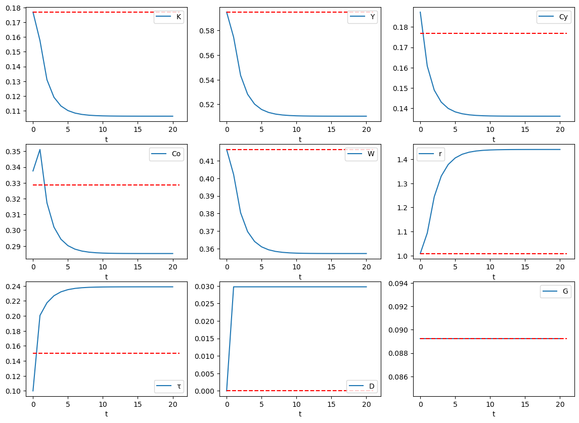
We first examine that the “guess and verify” method leads to the same numerical results as we obtain with the closed form solution when lump sum taxes are muted
δy_seq = np.ones(T+2) * 0.
δo_seq = np.ones(T+2) * 0.

D_pol = np.zeros(T+2)
G_pol = np.ones(T+2) * G_hat

# tax cut
τ0 = τ_hat * (1 - 1/3)
D1 = D_hat * (1 + r_hat * (1 - τ0)) + G_hat - τ0 * Y_hat - δy_seq[0] - δo_seq[0]
D_pol[0] = D_hat
D_pol[1:] = D1
quant_seq3, price_seq3, policy_seq3 = ak2.simulate(T, init_ss,
                                                   δy_seq, δo_seq,
                                                   D_pol=D_pol, G_pol=G_pol,
                                                   verbose=True)
Converge using 10 iterations

ak2.plot()
Next, we activate lump sum taxes.
Let’s alter our Experiment 1: Tax cut fiscal policy experiment by assuming that the government also increases lump sum taxes for both young and old people \(\delta_{yt}=\delta_{ot}=0.005, t\geq0\).
δy_seq = np.ones(T+2) * 0.005
δo_seq = np.ones(T+2) * 0.005

D1 = D_hat * (1 + r_hat * (1 - τ0)) + G_hat - τ0 * Y_hat - δy_seq[0] - δo_seq[0]
D_pol[1:] = D1

quant_seq4, price_seq4, policy_seq4 = ak2.simulate(T, init_ss,
                                                   δy_seq, δo_seq,
                                                   D_pol=D_pol, G_pol=G_pol)
Note how “crowding out” has been mitigated.
fig, axs = plt.subplots(3, 3, figsize=(14, 10))

# quantities
for i, name in enumerate(['K', 'Y', 'Cy', 'Co']):
    ax = axs[i//3, i%3]
    ax.plot(range(T+1), quant_seq3[:T+1, i], label=rf'{name}, $\delta$s=0')
    ax.plot(range(T+1), quant_seq4[:T+1, i], label=rf'{name}, $\delta$s=0.005')
    ax.hlines(init_ss[i], 0, T+1, color='r', linestyle='--')
    ax.legend()
    ax.set_xlabel('t')

# prices
for i, name in enumerate(['W', 'r']):
    ax = axs[(i+4)//3, (i+4)%3]
    ax.plot(range(T+1), price_seq3[:T+1, i], label=rf'{name}, $\delta$s=0')
    ax.plot(range(T+1), price_seq4[:T+1, i], label=rf'{name}, $\delta$s=0.005')
    ax.hlines(init_ss[i+4], 0, T+1, color='r', linestyle='--')
    ax.legend()
    ax.set_xlabel('t')

# policies
for i, name in enumerate(['τ', 'D', 'G']):
    ax = axs[(i+6)//3, (i+6)%3]
    ax.plot(range(T+1), policy_seq3[:T+1, i], label=rf'{name}, $\delta$s=0')
    ax.plot(range(T+1), policy_seq4[:T+1, i], label=rf'{name}, $\delta$s=0.005')
    ax.hlines(init_ss[i+6], 0, T+1, color='r', linestyle='--')
    ax.legend()
    ax.set_xlabel('t')
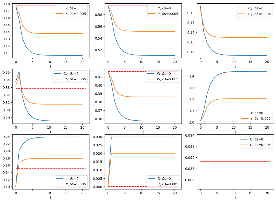
Comparing to Experiment 1: Tax cut, the government raises lump-sum taxes to finance the increasing debt interest payment, which is less distortionary comparing to raising the capital income tax rate.
