101. Optimal Misspecified Beliefs#
101.1. Overview#
This lecture continues the study of Phillips curve tradeoffs.
It follows chapter 6 of [Sargent, 1999].
In Adaptive Expectations and the Phelps Problem the public forecast inflation with a fixed adaptive rule whose parameter \(\lambda\) we simply chose.
That was unsatisfying in a way the vindication story of The Rise and Fall of U.S. Inflation cannot afford: a free parameter describing expectations is exactly what rational expectations was meant to eliminate.
Here we take the first step toward earning that parameter, by letting agents choose it to fit the data their own beliefs generate.
We describe three conceptual issues that recur throughout this suite of lectures:
how to formulate equilibria in which agents share a common misspecified least squares forecasting model,
how expectations can contribute independent dynamics within equilibria, and
how the classic adaptive expectations scheme can use second moments to approximate a first moment.
To expose these issues we temporarily set aside the Phillips curve and work with [Bray, 1982]’s simple model of the price of a single good, a workhorse for studying bounded rationality.
We alter Bray’s model to illustrate an equilibrium concept that merges aspects of rational and adaptive expectations in a new way, and that we apply to the Phillips curve in Self-Confirming Equilibria.
The focus is on market equilibrium with optimal but misspecified forecasts.
Optimal means the free parameters of the forecasting scheme are chosen by (nonlinear) least squares.
Misspecified means the forecasting model is wrong in functional form.
A distinctive feature is that the true model depends on how the agents’ model is misspecified: agents’ beliefs affect their behavior, which shapes the data they then fit.
We work in the frequency domain, so let’s import what we need:
import matplotlib.pyplot as plt
import numpy as np
from scipy.optimize import minimize_scalar
101.2. An experiment in Bray’s lab#
Following [Bray, 1982], assume that
where \(u_t\) is IID with mean zero and variance \(\sigma_u^2\), \(a > 0\), \(b \in (0, 1)\), \(p_t\) is the market price, and \(p_{t+1}^e\) is the market’s expectation of next period’s price.
The rational expectations equilibrium has \(p_{t+1}^e = \frac{a}{1-b}\) and \(p_t = \frac{a}{1-b} + u_t\).
Bray posited that \(p_{t+1}^e\) is the empirical average of past prices, and showed that when \(0 < b < 1\) this decreasing-gain scheme converges almost surely to the rational expectation \(\frac{a}{1-b}\).
During the transition, the state variable \(p_t^e\) contributes dynamics and makes the price serially correlated, but these dynamics are transitory: at the rational expectations equilibrium, \(p_t\) is a constant plus a serially uncorrelated shock.
101.2.1. Constant-gain adaptive expectations#
To let expectations impart persistent serial correlation, we depart from Bray and assume that the market has constant-gain adaptive expectations,
Bray’s scheme replaces \(C\) by \(\frac{1}{t}\), so that \(p_{t+1}^e\) becomes a sample average.
Fixing \(C\) instead discounts past observations, which arrests convergence to rational expectations and prevents \(p_{t+1}^e\) from converging to a constant.
Written as a distributed lag,
where \(L\) is the lag operator.
Equation (101.2) would be the linear least squares forecast if the price followed the integrated moving-average process
so the market perceives the price as composed of purely permanent and transitory components.
101.2.2. The actual law of motion#
Substituting the belief (101.3) into (101.1) shows that when the market forecasts this way, its actions make the actual law of motion for the price
where \(\nu = \frac{a}{1-b}\) and \(f(L)\) is defined to match.
The price has mean \(\nu\) and spectral density
Notice that \(F\) depends on \(C\) through \(f\).
Let’s encode the true process.
class BrayModel:
    """
    Bray's price model with constant-gain adaptive expectations.

    The perceived law of motion is an IMA(1,1) with unit root; to keep its
    spectral density well defined we approximate the unit root by a root ρ
    slightly below one, following Sargent (1999).
    """

    def __init__(self, a=1.0, b=0.5, σ_u=1.0, ρ=0.995, N=1024):
        self.a, self.b, self.σ_u, self.ρ, self.N = a, b, σ_u, ρ, N
        self.ν = a / (1 - b)
        ω = 2 * np.pi * np.arange(N) / N
        self.ω = ω
        self.z = np.exp(1j * ω)

    def true_spectrum(self, C):
        "Spectral density F(ω) of the actual price process, given belief C."
        b, z = self.b, self.z
        φ = (1 - C) / (1 - b * C)
        scale = 1 / (1 - b * C)
        f = scale * (1 - (1 - C) * z) / (1 - φ * z)
        return np.abs(f)**2 * self.σ_u**2

    def approx_spectrum(self, c, σ_ε2=1.0):
        "Spectral density G(ω) of the agent's approximating IMA model."
        g = (1 - (1 - c) * self.z) / (1 - self.ρ * self.z)
        return np.abs(g)**2 * σ_ε2
101.3. Optimal misspecification#
Two facts about the actual law (101.5) motivate an equilibrium restriction on \(C\):
Given that the price obeys (101.5), the true linear least squares one-step forecasting rule is not a geometric distributed lag like (101.2).
Even restricting the forecast to the form (101.2), the best such rule would make \(C\) solve a forecast-error-minimization problem, so \(C\) is an outcome, not a free parameter.
A rational expectations equilibrium would repair both features.
Following [Bray, 1982] we soften the equilibrium concept: we leave feature 1 untouched (agents keep the wrong functional form) while fixing feature 2 (they choose the best parameter within that form).
Think of putting a single individual into a market where everyone else (the “representative agent”) uses \(C\), so the price obeys (101.5).
The individual chooses \(c\) to fit the best model of the form
by minimizing the one-step-ahead forecast error variance.
Because \(g(L)\) has a unit root, its DC gain is infinite; this is exactly how the perceived model uses a unit root to fit the constant mean \(\nu\).
Numerically we replace the unit root by a root \(\rho\) slightly below one.
Definition 101.1 (Best-estimate map)
Given \(C\) and the consequent price process (101.5), the individual’s best forecast parameter \(c = B(C)\) is the nonlinear least squares estimator of \(c\) in (101.6), where the data are generated by (101.5).
Following the frequency-domain method of Hansen and Sargent [Hansen and Sargent, 1993], the best approximating \((c, \sigma_\epsilon^2)\) minimizes
where \(\omega_j = \frac{2\pi j}{N}\), and the term \(\frac{\nu^2}{G(0)}\) makes the approximating model use its near-unit-root to fit the mean.
Concentrating out \(\sigma_\epsilon^2\) leaves a one-dimensional minimization over \(c\).
Definition 101.2 (Equilibrium under forecast misspecification)
An equilibrium under forecast misspecification is a fixed point \(C = B(C)\).
At such a fixed point the representative agent is representative: the single individual’s best parameter equals the one everyone uses.
def best_estimate(model, C):
    "The best-estimate map c = B(C)."
    F = model.true_spectrum(C)
    z, ν, N = model.z, model.ν, model.N

    def neg_profile(c):
        H = np.abs((1 - (1 - c) * z) / (1 - model.ρ * z))**2   # |g|^2
        σ_ε2 = np.mean(F / H) + ν**2 / H[0]                    # concentrated
        return np.log(σ_ε2) + np.mean(np.log(H))               # profiled criterion

    res = minimize_scalar(neg_profile, bounds=(1e-4, 0.99), method='bounded')
    return res.x

def solve_equilibrium(model, C0=0.3, tol=1e-10, maxit=500):
    "Iterate the best-estimate map to a fixed point."
    C = C0
    for _ in range(maxit):
        C_new = best_estimate(model, C)
        if abs(C_new - C) < tol:
            break
        C = C_new
    return C_new
bray = BrayModel(a=1.0, b=0.5, σ_u=1.0)
C_star = solve_equilibrium(bray)
print(f"equilibrium belief   C = {C_star:.4f}")
equilibrium belief C = 0.0805
For these parameters the equilibrium belief is \(C \approx 0.08\), reproducing the value reported in chapter 6 of [Sargent, 1999].
Let’s also report the actual one-step-ahead forecast error standard deviation that agents incur by using their misspecified model.
def fitted_sigma2(model, C, c):
    "Concentrated innovation variance σ_ε^2 of the approximating model."
    F = model.true_spectrum(C)
    H = np.abs((1 - (1 - c) * model.z) / (1 - model.ρ * model.z))**2
    return np.mean(F / H) + model.ν**2 / H[0]

c_star = best_estimate(bray, C_star)
σ_bar = np.sqrt(fitted_sigma2(bray, C_star, c_star))
print(f"actual one-step forecast error std  σ̄_ε = {σ_bar:.4f}")
actual one-step forecast error std σ̄_ε = 1.0579
101.4. Comparing the true and forecasting models#
For the equilibrium \(C\), we plot the equilibrium spectral densities of the true and approximating models.
F = bray.true_spectrum(C_star)
σ_ε2 = fitted_sigma2(bray, C_star, c_star)
G = bray.approx_spectrum(c_star, σ_ε2)

half = bray.N // 2
fig, ax = plt.subplots(figsize=(8, 5))
ax.plot(bray.ω[:half], np.log(F[:half]), 'C0', label='true model', lw=2)
ax.plot(bray.ω[:half], np.log(G[:half]), 'C1--', label='forecasting model', lw=2)
ax.set_xlabel(r'angular frequency $\omega$')
ax.set_ylabel('log spectral density')
ax.legend()
plt.show()
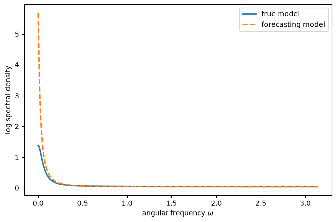
Fig. 101.1 Spectral densities of the true price process and of the agents’ approximating model#
In minimizing (101.7), the approximating model uses its near-unit-root to fit the mean.
The large gap between the spectral densities at low frequencies reflects how the approximating model fits a first moment (the mean \(\nu\)) with features of second moments (a spike in the spectral density at frequency zero).
The true spectral density decreases sharply with frequency — Granger’s “typical spectral shape” [Granger, 1966] — revealing substantial positive serial correlation in the price, because agents’ belief that the price is subject to permanent shocks makes shocks persist.
101.4.1. Impulse responses#
We compare the impulse response functions of the two models by feeding a unit shock through each moving-average representation.
def impulse_response(num_roots, den_roots, T=25):
    "IRF of (1 - num L)/(1 - den L): coefficients of the ratio of lag polys."
    h = np.empty(T)
    h[0] = 1.0
    for k in range(1, T):
        h[k] = den_roots * h[k - 1]
    h[1:] -= num_roots * h[:-1]           # apply the numerator (1 - num L)
    return h

φ = (1 - C_star) / (1 - bray.b * C_star)
scale = 1 / (1 - bray.b * C_star)
irf_true = scale * impulse_response(1 - C_star, φ)          # f(L)
irf_approx = impulse_response(1 - c_star, bray.ρ)           # g(L)

fig, ax = plt.subplots(figsize=(8, 5))
ax.plot(irf_true, 'C0o-', ms=4, label='true model', lw=2)
ax.plot(irf_approx, 'C1s--', ms=4, label='approximating model', lw=2)
ax.set_xlabel('lag')
ax.set_ylabel('response')
ax.legend()
plt.show()
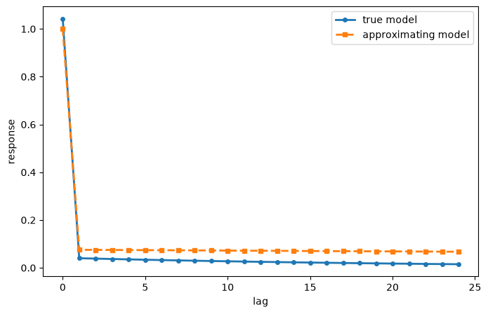
Fig. 101.2 Impulse responses of the true and approximating models#
The impulse response of the true model affirms the serial correlation in the price.
The approximating model tends to under-predict the short-term consequences of a shock while over-predicting the long-term ones: its near-unit-root produces a response that does not die out.
101.5. Lessons#
The agents in this model are boundedly rational: rational describes their use of least squares, and bounded describes their model misspecification.
Under rational expectations there is only one model in play.
Under bounded rationality there must be at least two: the one used by the boundedly rational agents, and the true one.
These mutually influence each other — the boundedly rational agents use their model to approximate the true one, and the true one reflects the decisions of the agents — and both differ from the rational expectations model.
The peculiar way that the adaptive expectations model uses a unit root to mimic a constant foreshadows a version of the Phillips curve model, developed in Self-Confirming Equilibria, that will help vindicate econometric policy evaluation.
This same trick — using a unit root to approximate a constant — turns out to be the engine of the escape dynamics of Adaptive Learning and Escape Dynamics and Escaping Nash Inflation, where a learning government’s estimated Phillips curve drifts toward the induction hypothesis and, believing it, cuts inflation toward Ramsey.
101.6. Exercises#
Exercise 101.1
The equilibrium belief \(C\) depends on the feedback parameter \(b\) in (101.1).
Compute and plot the equilibrium \(C\) as a function of \(b\) over a grid \(b \in \{0.1, 0.2, \ldots, 0.8\}\), holding \(a = 1\) and \(\sigma_u = 1\) fixed.
How does stronger expectational feedback (larger \(b\)) affect the equilibrium amount of discounting of past data?
Solution
b_grid = np.arange(0.1, 0.85, 0.1)
C_of_b = [solve_equilibrium(BrayModel(a=1.0, b=b, σ_u=1.0)) for b in b_grid]

fig, ax = plt.subplots(figsize=(8, 4.5))
ax.plot(b_grid, C_of_b, 'o-', lw=2)
ax.set_xlabel('feedback parameter $b$')
ax.set_ylabel('equilibrium belief $C$')
ax.set_title('Equilibrium belief by expectational feedback')
plt.show()
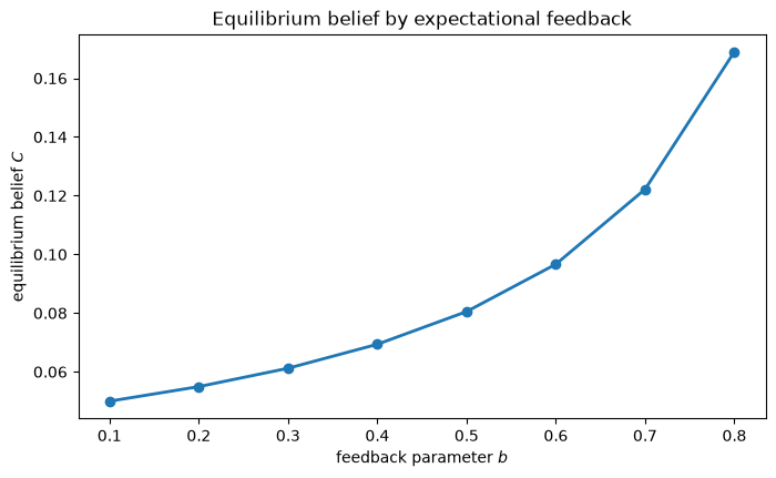
Stronger feedback raises the equilibrium gain \(C\): agents put more weight on recent observations, so the price process they generate is less persistent than it would otherwise be.
Exercise 101.2
Verify that the equilibrium is a genuine fixed point by plotting the best-estimate map \(c = B(C)\) against the 45-degree line, and mark the fixed point.
Solution
C_grid = np.linspace(0.02, 0.4, 25)
B_vals = [best_estimate(bray, C) for C in C_grid]

fig, ax = plt.subplots(figsize=(6, 6))
ax.plot(C_grid, B_vals, 'C0', label='$B(C)$')
ax.plot(C_grid, C_grid, 'k--', lw=1, label='45 degrees')
ax.plot(C_star, C_star, 'ko')
ax.annotate('equilibrium', (C_star, C_star),
            (C_star + 0.05, C_star - 0.03))
ax.set_xlabel('$C$')
ax.set_ylabel('$B(C)$')
ax.set_title('The best-estimate map and its fixed point')
ax.legend()
plt.show()
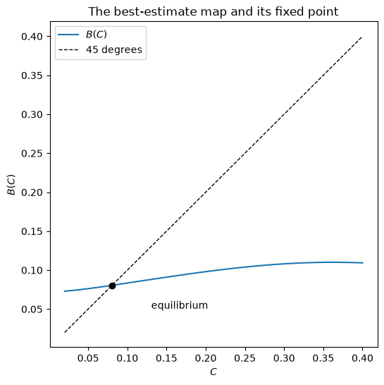
The best-estimate map crosses the 45-degree line at the equilibrium belief, confirming \(C = B(C)\).