29. Likelihood Ratio Processes and Bayesian Learning#
29.1. Overview#
This lecture describes the role that likelihood ratio processes play in Bayesian learning.
As in this lecture, we’ll use a simple statistical setting from this lecture.
We’ll focus on how a likelihood ratio process and a prior probability determine a posterior probability.
We’ll derive a convenient recursion for today’s posterior as a function of yesterday’s posterior and today’s multiplicative increment to a likelihood process.
We’ll also present a useful generalization of that formula that represents today’s posterior in terms of an initial prior and today’s realization of the likelihood ratio process.
We’ll study how, at least in our setting, a Bayesian eventually learns the probability distribution that generates the data, an outcome that rests on the asymptotic behavior of likelihood ratio processes studied in this lecture.
We’ll also drill down into the psychology of our Bayesian learner and study dynamics under his subjective beliefs.
This lecture provides technical results that underly outcomes to be studied in this lecture and this lecture and this lecture.
We’ll begin by loading some Python modules.
import matplotlib.pyplot as plt
import numpy as np
from numba import vectorize, jit, prange
from math import gamma
import pandas as pd
from scipy.integrate import quad


import seaborn as sns
colors = sns.color_palette()

@jit
def set_seed():
    np.random.seed(142857)
set_seed()
29.2. The Setting#
We begin by reviewing the setting in this lecture, which we adopt here too.
A nonnegative random variable \(W\) has one of two probability density functions, either \(f\) or \(g\).
Before the beginning of time, nature once and for all decides whether she will draw a sequence of IID draws from \(f\) or from \(g\).
We will sometimes let \(q\) be the density that nature chose once and for all, so that \(q\) is either \(f\) or \(g\), permanently.
Nature knows which density it permanently draws from, but we the observers do not.
We do know both \(f\) and \(g\), but we don’t know which density nature chose.
But we want to know.
To do that, we use observations.
We observe a sequence \(\{w_t\}_{t=1}^T\) of \(T\) IID draws from either \(f\) or \(g\).
We want to use these observations to infer whether nature chose \(f\) or \(g\).
A likelihood ratio process is a useful tool for this task.
To begin, we define the key component of a likelihood ratio process, namely, the time \(t\) likelihood ratio as the random variable
We assume that \(f\) and \(g\) both put positive probabilities on the same intervals of possible realizations of the random variable \(W\).
That means that under the \(g\) density, \(\ell (w_t)= \frac{f\left(w_{t}\right)}{g\left(w_{t}\right)}\) is evidently a nonnegative random variable with mean \(1\).
A likelihood ratio process for sequence \(\left\{ w_{t}\right\} _{t=1}^{\infty}\) is defined as
where \(w^t=\{ w_1,\dots,w_t\}\) is a history of observations up to and including time \(t\).
Sometimes for shorthand we’ll write
where we use the conventions that \(f(w^t) = f(w_1) f(w_2) \ldots f(w_t)\) and \(g(w^t) = g(w_1) g(w_2) \ldots g(w_t)\).
Notice that the likelihood process satisfies the recursion or multiplicative decomposition
The likelihood ratio and its logarithm are key tools for making inferences using a classic frequentist approach due to Neyman and Pearson [Neyman and Pearson, 1933].
We’ll again deploy the following Python code from this lecture that evaluates \(f\) and \(g\) as two different beta distributions, then computes and simulates an associated likelihood ratio process by generating a sequence \(w^t\) from some probability distribution, for example, a sequence of IID draws from \(g\).
# Parameters in the two beta distributions.
F_a, F_b = 1, 1
G_a, G_b = 3, 1.2

@vectorize
def p(x, a, b):
    r = gamma(a + b) / (gamma(a) * gamma(b))
    return r * x** (a-1) * (1 - x) ** (b-1)

# The two density functions.
f = jit(lambda x: p(x, F_a, F_b))
g = jit(lambda x: p(x, G_a, G_b))
@jit
def simulate(a, b, T=50, N=500):
    '''
    Generate N sets of T observations of the likelihood ratio,
    return as N x T matrix.

    '''

    l_arr = np.empty((N, T))

    for i in range(N):

        for j in range(T):
            w = np.random.beta(a, b)
            l_arr[i, j] = f(w) / g(w)

    return l_arr
We’ll also use the following Python code to prepare some informative simulations
l_arr_g = simulate(G_a, G_b, N=50000)
l_seq_g = np.cumprod(l_arr_g, axis=1)
l_arr_f = simulate(F_a, F_b, N=50000)
l_seq_f = np.cumprod(l_arr_f, axis=1)
29.3. Likelihood Ratio Processes and Bayes’ Law#
Let \(\pi_0 \in [0,1]\) be a Bayesian statistician’s prior probability that nature generates \(w^t\) as a sequence of i.i.d. draws from distribution \(f\).
here “probability” is to be interpreted as a way to summarize or express a subjective opinion
it does not mean an anticipated relative frequency as sample size grows without limit
Let \(\pi_{t+1}\) be a Bayesian posterior probability defined as
The likelihood ratio process is a principal actor in the formula that governs the evolution of the posterior probability \(\pi_t\), an instance of Bayes’ Law.
Let’s derive a couple of formulas for \(\pi_{t+1}\), one in terms of likelihood ratio \(l(w_t)\), the other in terms of \(L(w^t)\).
To begin, we use the notational conventions
\(f(w^{t+1}) \equiv f(w_1) f(w_2) \cdots f(w_{t+1})\)
\(g(w^{t+1}) \equiv g(w_1) g(w_2) \cdots g(w_{t+1})\)
\(\pi_0 ={\rm Prob}(q=f |\emptyset)\)
\(\pi_t = {\rm Prob}(q=f |w^t)\)
Here the symbol \(\emptyset\) means “empty set” or “no data”.
With no data in hand, our Bayesian statistician thinks that the probability density of the sequence \(w^{t+1}\) is
Laws of probability say that the joint distribution \({\rm Prob}(AB)\) of events \(A\) and \(B\) are connected to the conditional distributions \({\rm Prob}(A |B)\) and \({\rm Prob}(B |A)\) by
We are interested in events
where braces \(\{\cdot\}\) are our shorthand for “event”.
So in our setting, probability laws (29.2) imply that
or
or
Dividing both the numerator and the denominator on the right side of the above equation by \(g(w^{t+1})\) implies
Formula (29.3) can be regarded as a one step revision of prior probability \(\pi_0\) after seeing the batch of data \(\left\{ w_{i}\right\} _{i=1}^{t+1}\).
Formula (29.3) shows the key role that the likelihood ratio process \(L\left(w^{t+1}\right)\) plays in determining the posterior probability \(\pi_{t+1}\).
Formula (29.3) is the foundation for the insight that, because of how the likelihood ratio process behaves as \(t \rightarrow + \infty\), the likelihood ratio process dominates the initial prior \(\pi_0\) in determining the limiting behavior of \(\pi_t\).
29.3.1. A recursive formula#
We can use a similar line of argument to get a recursive version of formula (29.3).
The laws of probability imply
or
Evidently, the above equation asserts that
Dividing both the numerator and the denominator on the right side of the equation (29.4) by \(g(w_{t+1})\) implies the recursion
with \(\pi_{0}\) being a Bayesian prior probability that \(q = f\), i.e., a personal or subjective belief about \(q\) based on our having seen no data.
Formula (29.3) can be deduced by iterating on equation (29.5).
Below we define a Python function that updates belief \(\pi\) using likelihood ratio \(\ell\) according to recursion (29.5)
@jit
def update(π, l):
    "Update π using likelihood l"

    # Update belief
    π = π * l / (π * l + 1 - π)

    return π
As mentioned above, formula (29.3) shows the key role that the likelihood ratio process \(L\left(w^{t+1}\right)\) plays in determining the posterior probability \(\pi_{t+1}\).
As \(t \rightarrow + \infty\), the likelihood ratio process dominates the initial prior \(\pi_0\) in determining the limiting behavior of \(\pi_t\).
To illustrate this insight, below we will plot graphs showing one simulated path of the likelihood ratio process \(L_t\) along with two paths of \(\pi_t\) that are associated with the same realization of the likelihood ratio process but different initial prior probabilities \(\pi_{0}\).
First, we tell Python two values of \(\pi_0\).
π1, π2 = 0.2, 0.8
Next we generate paths of the likelihood ratio process \(L_t\) and the posterior \(\pi_t\) for a history of IID draws from density \(f\).
T = l_arr_f.shape[1]
π_seq_f = np.empty((2, T+1))
π_seq_f[:, 0] = π1, π2

for t in range(T):
    for i in range(2):
        π_seq_f[i, t+1] = update(π_seq_f[i, t], l_arr_f[0, t])
fig, ax1 = plt.subplots()

for i in range(2):
    ax1.plot(range(T+1), π_seq_f[i, :], label=fr"$\pi_0$={π_seq_f[i, 0]}")

ax1.set_ylabel(r"$\pi_t$")
ax1.set_xlabel("t")
ax1.legend()
ax1.set_title("when f governs data")

ax2 = ax1.twinx()
ax2.plot(range(1, T+1), np.log(l_seq_f[0, :]), '--', color='b')
ax2.set_ylabel("$log(L(w^{t}))$")

plt.show()
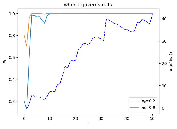
The dotted line in the graph above records the logarithm of the likelihood ratio process \(\log L(w^t)\).
Please note that there are two different scales on the \(y\) axis.
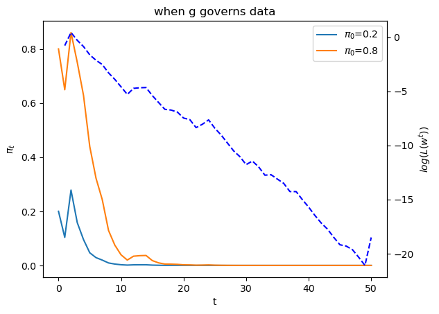
Now let’s study what happens when the history consists of IID draws from density \(g\)
T = l_arr_g.shape[1]
π_seq_g = np.empty((2, T+1))
π_seq_g[:, 0] = π1, π2

for t in range(T):
    for i in range(2):
        π_seq_g[i, t+1] = update(π_seq_g[i, t], l_arr_g[0, t])
fig, ax1 = plt.subplots()

for i in range(2):
    ax1.plot(range(T+1), π_seq_g[i, :], label=fr"$\pi_0$={π_seq_g[i, 0]}")

ax1.set_ylabel(r"$\pi_t$")
ax1.set_xlabel("t")
ax1.legend()
ax1.set_title("when g governs data")

ax2 = ax1.twinx()
ax2.plot(range(1, T+1), np.log(l_seq_g[0, :]), '--', color='b')
ax2.set_ylabel("$log(L(w^{t}))$")

plt.show()
Below we offer Python code that verifies that nature chose permanently to draw from density \(f\).
π_seq = np.empty((2, T+1))
π_seq[:, 0] = π1, π2

for i in range(2):
    πL = π_seq[i, 0] * l_seq_f[0, :]
    π_seq[i, 1:] = πL / (πL + 1 - π_seq[i, 0])
np.abs(π_seq - π_seq_f).max() < 1e-10
np.True_
We thus conclude that the likelihood ratio process is a key ingredient of the formula (29.3) for a Bayesian’s posterior probability that nature has drawn history \(w^t\) as repeated draws from density \(f\).
29.4. Another timing protocol#
Let’s study how the posterior probability \(\pi_t = {\rm Prob}(q=f|w^{t}) \) behaves when nature generates the history \(w^t = \{w_1, w_2, \dots, w_t\}\) under a different timing protocol.
Until now we assumed that before time \(1\) nature somehow chose to draw \(w^t\) as an iid sequence from either \(f\) or \(g\).
Nature’s decision about whether to draw from \(f\) or \(g\) was thus permanent.
We now assume a different timing protocol in which before each period \(t =1, 2, \ldots\) nature
flips an \(x\)-weighted coin, then
draws from \(f\) if it has drawn a “head”
draws from \(g\) if it has drawn a “tail”.
Under this timing protocol, nature draws permanently from neither \(f\) nor \(g\), so a statistician who thinks that nature is drawing i.i.d. draws permanently from one of them is mistaken.
in truth, nature actually draws permanently from an \(x\)-mixture of \(f\) and \(g\) – a distribution that is neither \(f\) nor \(g\) when \(x \in (0,1)\)
Thus, the Bayesian prior \(\pi_0\) and the sequence of posterior probabilities described by equation (29.3) should not be interpreted as the statistician’s opinion about the mixing parameter \(x\) under the alternative timing protocol in which nature draws from an \(x\)-mixture of \(f\) and \(g\).
This is clear when we remember the definition of \(\pi_t\) in equation (29.1), which for convenience we repeat here:
Let’s write some Python code to study how \(\pi_t\) behaves when nature actually generates data as i.i.d. draws from neither \(f\) nor from \(g\) but instead as i.i.d. draws from an \(x\)-mixture of two beta distributions.
Note
This is a situation in which the statistician’s model is misspecified, so we should anticipate that a Kullback-Liebler divergence with respect to an \(x\)-mixture distribution will shape outcomes.
We can study how \(\pi_t\) would behave for various values of nature’s mixing probability \(x\).
First, let’s create a function to simulate data under the mixture timing protocol:
@jit
def simulate_mixture_path(x_true, T):
    """
    Simulate T observations under mixture timing protocol.
    """
    w = np.empty(T)
    for t in range(T):
        if np.random.rand() < x_true:
            w[t] = np.random.beta(F_a, F_b)
        else:
            w[t] = np.random.beta(G_a, G_b)
    return w
Let’s generate a sequence of observations from this mixture model with a true mixing probability of \(x=0.5\).
We will first use this sequence to study how \(\pi_t\) behaves.
Note
Later, we can use it to study how a statistician who knows that nature generates data from an \(x\)-mixture of \(f\) and \(g\) could construct maximum likelihood or Bayesian estimators of \(x\) along with the free parameters of \(f\) and \(g\).
x_true = 0.5
T_mix = 200

# Three different priors with means 0.25, 0.5, 0.75
prior_params = [(1, 3), (1, 1), (3, 1)]
prior_means = [a/(a+b) for a, b in prior_params]

# Generate one path of observations from the mixture
set_seed()
w_mix = simulate_mixture_path(x_true, T_mix)
29.4.1. Behavior of \(\pi_t\) under wrong model#
Let’s study how the posterior probability \(\pi_t\) that nature permanently draws from \(f\) behaves when data are actually generated by an \(x\)-mixture of \(f\) and \(g\).
fig, ax = plt.subplots(figsize=(10, 6))
T_plot = 200

for i, mean0 in enumerate(prior_means):
    π_wrong = np.empty(T_plot + 1)
    π_wrong[0] = mean0

    # Compute likelihood ratios for the mixture data
    for t in range(T_plot):
        l_t = f(w_mix[t]) / g(w_mix[t])
        π_wrong[t + 1] = update(π_wrong[t], l_t)

    ax.plot(range(T_plot + 1), π_wrong,
            label=fr'$\pi_0 = ${mean0:.2f}',
            color=colors[i], linewidth=2)

ax.axhline(y=x_true, color='black', linestyle='--',
           label=f'True x = {x_true}', linewidth=2)
ax.set_xlabel('t')
ax.set_ylabel(r'$\pi_t$')
ax.legend()
plt.show()
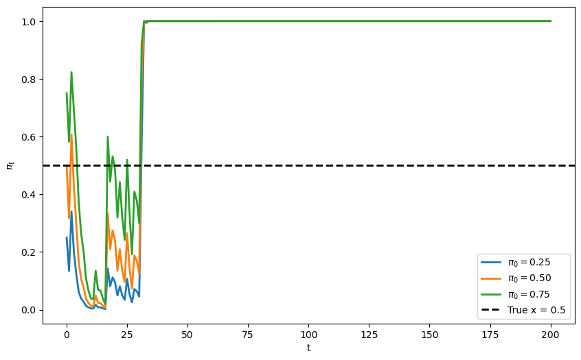
Evidently, \(\pi_t\) converges to 1.
This indicates that the model concludes that the data is generated by \(f\).
Why does this happen?
Given \(x = 0.5\), the data generating process is a mixture of \(f\) and \(g\): \(m(w) = \frac{1}{2}f(w) + \frac{1}{2}g(w)\).
Let’s check the KL divergence of the mixture distribution \(m\) from both \(f\) and \(g\).
def compute_KL(f, g):
    """
    Compute KL divergence KL(f, g)
    """
    integrand = lambda w: f(w) * np.log(f(w) / g(w))
    val, _ = quad(integrand, 1e-5, 1-1e-5)
    return val


def compute_div_m(f, g):
    """
    Compute Jensen-Shannon divergence
    """
    def m(w):
        return 0.5 * (f(w) + g(w))

    return compute_KL(m, f), compute_KL(m, g)


KL_f, KL_g = compute_div_m(f, g)

print(f'KL(m, f) = {KL_f:.3f}\nKL(m, g) = {KL_g:.3f}')
KL(m, f) = 0.073
KL(m, g) = 0.281
Since \(KL(m, f) < KL(m, g)\), \(f\) is “closer” to the mixture distribution \(m\).
Hence by our discussion on KL divergence and likelihood ratio process in Likelihood Ratio Processes, \(\log(L_t) \to \infty\) as \(t \to \infty\).
Now looking back to the key equation (29.3).
Consider the function
The limit \(\lim_{z \to \infty} h(z)\) is 1.
Hence \(\pi_t \to 1\) as \(t \to \infty\) for any \(\pi_0 \in (0,1)\).
This explains what we observed in the plot above.
But how can we learn the true mixing parameter \(x\)?
This topic is taken up in Incorrect Models.
We explore how to learn the true mixing parameter \(x\) in the exercise of Incorrect Models.
29.5. Behavior of Posterior Probability \(\{\pi_t\}\) Under Subjective Probability Distribution#
We’ll end this lecture by briefly studying what our Bayesian learner expects to learn under the subjective beliefs \(\pi_t\) cranked out by Bayes’ law.
This will provide us with some perspective on our application of Bayes’s law as a theory of learning.
As we shall see, at each time \(t\), the Bayesian learner knows that he will be surprised.
But he expects that new information will not lead him to change his beliefs.
And it won’t on average under his subjective beliefs.
We’ll continue with our setting in which a McCall worker knows that successive draws of his wage are drawn from either \(F\) or \(G\), but does not know which of these two distributions nature has drawn once-and-for-all before time \(0\).
We’ll review and reiterate and rearrange some formulas that we have encountered above and in associated lectures.
The worker’s initial beliefs induce a joint probability distribution over a potentially infinite sequence of draws \(w_0, w_1, \ldots \).
Bayes’ law is simply an application of laws of probability to compute the conditional distribution of the \(t\)th draw \(w_t\) conditional on \([w_0, \ldots, w_{t-1}]\).
After our worker puts a subjective probability \(\pi_{-1}\) on nature having selected distribution \(F\), we have in effect assumed from the start that the decision maker knows the joint distribution for the process \(\{w_t\}_{t=0}\).
We assume that the worker also knows the laws of probability theory.
A respectable view is that Bayes’ law is less a theory of learning than a statement about the consequences of information inflows for a decision maker who thinks he knows the truth (i.e., a joint probability distribution) from the beginning.
29.5.1. Mechanical details again#
At time \(0\) before drawing a wage offer, the worker attaches probability \(\pi_{-1} \in (0,1)\) to the distribution being \(F\).
Before drawing a wage at time \(0\), the worker thus believes that the density of \(w_0\) is
Let \(a \in \{ f, g\} \) be an index that indicates whether nature chose permanently to draw from distribution \(f\) or from distribution \(g\).
After drawing \(w_0\), the worker uses Bayes’ law to deduce that the posterior probability \(\pi_0 = {\rm Prob}({a = f | w_0}) \) that the density is \(f(w)\) is
More generally, after making the \(t\)th draw and having observed \(w_t, w_{t-1}, \ldots, w_0\), the worker believes that the probability that \(w_{t+1}\) is being drawn from distribution \(F\) is
or
and that the density of \(w_{t+1}\) conditional on \(w_t, w_{t-1}, \ldots, w_0\) is
Notice that
so that the process \(\pi_t\) is a martingale.
Indeed, it is a bounded martingale because each \(\pi_t\), being a probability, is between \(0\) and \(1\).
In the first line in the above string of equalities, the term in the first set of brackets is just \(\pi_t\) as a function of \(w_{t}\), while the term in the second set of brackets is the density of \(w_{t}\) conditional on \(w_{t-1}, \ldots , w_0\) or equivalently conditional on the sufficient statistic \(\pi_{t-1}\) for \(w_{t-1}, \ldots , w_0\).
Notice that here we are computing \(E(\pi_t | \pi_{t-1})\) under the subjective density described in the second term in brackets.
Because \(\{\pi_t\}\) is a bounded martingale sequence, it follows from the martingale convergence theorem that \(\pi_t\) converges almost surely to a random variable in \([0,1]\).
Practically, this means that probability one is attached to sample paths \(\{\pi_t\}_{t=0}^\infty\) that converge.
According to the theorem, different sample paths can converge to different limiting values.
Thus, let \(\{\pi_t(\omega)\}_{t=0}^\infty\) denote a particular sample path indexed by a particular \(\omega \in \Omega\).
We can think of nature as drawing an \(\omega \in \Omega\) from a probability distribution \({\textrm{Prob}} \Omega\) and then generating a single realization (or simulation) \(\{\pi_t(\omega)\}_{t=0}^\infty\) of the process.
The limit points of \(\{\pi_t(\omega)\}_{t=0}^\infty\) as \(t \rightarrow +\infty\) are realizations of a random variable that is swept out as we sample \(\omega\) from \(\Omega\) and construct repeated draws of \(\{\pi_t(\omega)\}_{t=0}^\infty\).
By staring at law of motion (29.5) or (29.6) , we can figure out some things about the probability distribution of the limit points
Evidently, since the likelihood ratio \(\ell(w_t) \) differs from \(1\) when \(f \neq g\), as we have assumed, the only possible fixed points of (29.6) are
and
Thus, for some realizations, \(\lim_{\rightarrow + \infty} \pi_t(\omega) =1\) while for other realizations, \(\lim_{\rightarrow + \infty} \pi_t(\omega) =0\).
Now let’s remember that \(\{\pi_t\}_{t=0}^\infty\) is a martingale and apply the law of iterated expectations.
The law of iterated expectations implies
and in particular
Applying the above formula to \(\pi_\infty\), we obtain
where the mathematical expectation \(E_{-1}\) here is taken with respect to the probability measure \({\textrm{Prob}(\Omega)}\).
Since the only two values that \(\pi_\infty(\omega)\) can take are \(1\) and \(0\), we know that for some \(\lambda \in [0,1]\)
and consequently that
Combining this equation with equation (20), we deduce that the probability that \({\textrm{Prob}(\Omega)}\) attaches to \(\pi_\infty(\omega)\) being \(1\) must be \(\pi_{-1}\).
Thus, under the worker’s subjective distribution, \(\pi_{-1}\) of the sample paths of \(\{\pi_t\}\) will converge pointwise to \(1\) and \(1 - \pi_{-1}\) of the sample paths will converge pointwise to \(0\).
29.5.2. Some simulations#
Let’s watch the martingale convergence theorem at work in some simulations of our learning model under the worker’s subjective distribution.
Let us simulate \(\left\{ \pi_{t}\right\} _{t=0}^{T}\), \(\left\{ w_{t}\right\} _{t=0}^{T}\) paths where for each \(t\geq0\), \(w_t\) is drawn from the subjective distribution
We’ll plot a large sample of paths.
@jit
def martingale_simulate(π0, N=5000, T=200):

    π_path = np.empty((N,T+1))
    w_path = np.empty((N,T))
    π_path[:,0] = π0

    for n in range(N):
        π = π0
        for t in range(T):
            # draw w
            if np.random.rand() <= π:
                w = np.random.beta(F_a, F_b)
            else:
                w = np.random.beta(G_a, G_b)
            π = π*f(w)/g(w)/(π*f(w)/g(w) + 1 - π)
            π_path[n,t+1] = π
            w_path[n,t] = w

    return π_path, w_path

def fraction_0_1(π0, N, T, decimals):

    π_path, w_path = martingale_simulate(π0, N=N, T=T)
    values, counts = np.unique(np.round(π_path[:,-1], decimals=decimals), return_counts=True)
    return values, counts

def create_table(π0s, N=10000, T=500, decimals=2):

    outcomes = []
    for π0 in π0s:
        values, counts = fraction_0_1(π0, N=N, T=T, decimals=decimals)
        freq = counts/N
        outcomes.append(dict(zip(values, freq)))
    table = pd.DataFrame(outcomes).sort_index(axis=1).fillna(0)
    table.index = π0s
    return table

# simulate
T = 200
π0 = .5

π_path, w_path = martingale_simulate(π0=π0, T=T, N=10000)
fig, ax = plt.subplots()
for i in range(100):
    ax.plot(range(T+1), π_path[i, :])

ax.set_xlabel('$t$')
ax.set_ylabel(r'$\pi_t$')
plt.show()
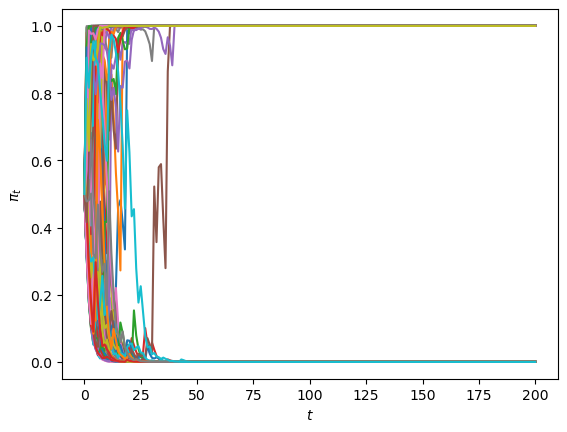
The above graph indicates that
each of paths converges
some of the paths converge to \(1\)
some of the paths converge to \(0\)
none of the paths converge to a limit point not equal to \(0\) or \(1\)
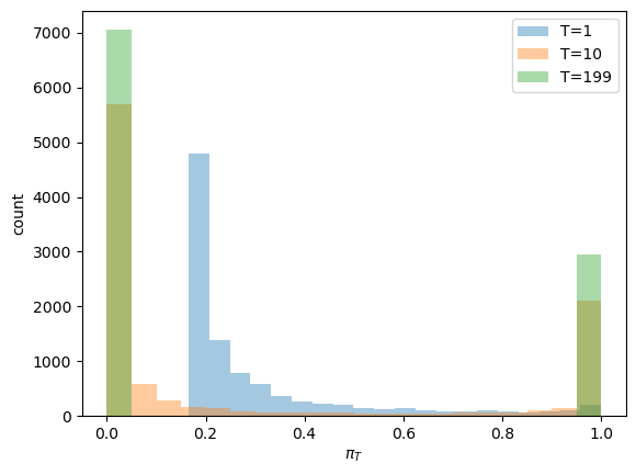
Convergence actually occurs pretty fast, as the following graph of the cross-ensemble distribution of \(\pi_t\) for various small \(t\)’s indicates.
fig, ax = plt.subplots()
for t in [1, 10, T-1]:
    ax.hist(π_path[:,t], bins=20, alpha=0.4, label=f'T={t}')

ax.set_ylabel('count')
ax.set_xlabel(r'$\pi_T$')
ax.legend(loc='lower right')
plt.show()
Evidently, by \(t = 199\), \(\pi_t\) has converged to either \(0\) or \(1\).
The fraction of paths that have converged to \(1\) is \(.5\)
The fractions of paths that have converged to \(0\) is also \(.5\).
Does the fraction \(.5\) ring a bell?
Yes, it does: it equals the value of \(\pi_0 = .5 \) that we used to generate each sequence in the ensemble.
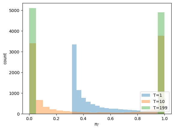
So let’s change \(\pi_0\) to \(.3\) and watch what happens to the distribution of the ensemble of \(\pi_t\)’s for various \(t\)’s.
# simulate
T = 200
π0 = .3

π_path3, w_path3 = martingale_simulate(π0=π0, T=T, N=10000)
fig, ax = plt.subplots()
for t in [1, 10, T-1]:
    ax.hist(π_path3[:,t], bins=20, alpha=0.4, label=f'T={t}')

ax.set_ylabel('count')
ax.set_xlabel(r'$\pi_T$')
ax.legend(loc='upper right')
plt.show()
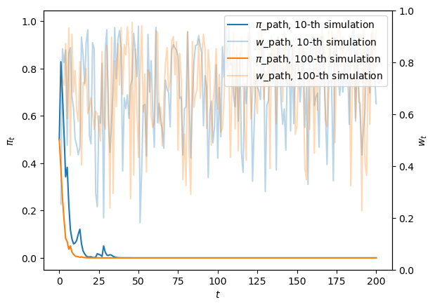
For the preceding ensemble that assumed \(\pi_0 = .5\), the following graph shows two paths of \(w_t\)’s and the \(\pi_t\) sequences that gave rise to them.
Notice that one of the paths involves systematically higher \(w_t\)’s, outcomes that push \(\pi_t\) upward.
The luck of the draw early in a simulation pushes the subjective distribution to draw from \(F\) more frequently along a sample path, and this pushes \(\pi_t\) toward \(0\).
fig, ax = plt.subplots()
for i, j in enumerate([10, 100]):
    ax.plot(range(T+1), π_path[j,:], color=colors[i], label=fr'$\pi$_path, {j}-th simulation')
    ax.plot(range(1,T+1), w_path[j,:], color=colors[i], label=fr'$w$_path, {j}-th simulation', alpha=0.3)

ax.legend(loc='upper right')
ax.set_xlabel('$t$')
ax.set_ylabel(r'$\pi_t$')
ax2 = ax.twinx()
ax2.set_ylabel("$w_t$")
plt.show()
29.6. Initial Prior is Verified by Paths Drawn from Subjective Conditional Densities#
Now let’s use our Python code to generate a table that checks out our earlier claims about the probability distribution of the pointwise limits \(\pi_{\infty}(\omega)\).
We’ll use our simulations to generate a histogram of this distribution.
In the following table, the left column in bold face reports an assumed value of \(\pi_{-1}\).
The second column reports the fraction of \(N = 10000\) simulations for which \(\pi_{t}\) had converged to \(0\) at the terminal date \(T=500\) for each simulation.
The third column reports the fraction of \(N = 10000\) simulations for which \(\pi_{t}\) had converged to \(1\) at the terminal date \(T=500\) for each simulation.
# create table
table = create_table(list(np.linspace(0,1,11)), N=10000, T=500)
table
| 0.0 | 1.0 | |
|---|---|---|
| 0.0 | 1.0000 | 0.0000 |
| 0.1 | 0.8984 | 0.1016 |
| 0.2 | 0.8000 | 0.2000 |
| 0.3 | 0.6981 | 0.3019 |
| 0.4 | 0.6004 | 0.3996 |
| 0.5 | 0.4968 | 0.5032 |
| 0.6 | 0.3995 | 0.6005 |
| 0.7 | 0.3007 | 0.6993 |
| 0.8 | 0.2074 | 0.7926 |
| 0.9 | 0.0964 | 0.9036 |
| 1.0 | 0.0000 | 1.0000 |
The fraction of simulations for which \(\pi_{t}\) had converged to \(1\) is indeed always close to \(\pi_{-1}\), as anticipated.
29.7. Drilling Down a Little Bit#
To understand how the local dynamics of \(\pi_t\) behaves, it is enlightening to consult the variance of \(\pi_{t}\) conditional on \(\pi_{t-1}\).
Under the subjective distribution this conditional variance is defined as
We can use a Monte Carlo simulation to approximate this conditional variance.
We approximate it for a grid of points \(\pi_{t-1} \in [0,1]\).
Then we’ll plot it.
@jit
def compute_cond_var(pi, mc_size=int(1e6)):
    # create monte carlo draws
    mc_draws = np.zeros(mc_size)

    for i in prange(mc_size):
        if np.random.rand() <= pi:
            mc_draws[i] = np.random.beta(F_a, F_b)
        else:
            mc_draws[i] = np.random.beta(G_a, G_b)

    dev = pi*f(mc_draws)/(pi*f(mc_draws) + (1-pi)*g(mc_draws)) - pi
    return np.mean(dev**2)

pi_array = np.linspace(0, 1, 40)
cond_var_array = []

for pi in pi_array:
    cond_var_array.append(compute_cond_var(pi))

fig, ax = plt.subplots()
ax.plot(pi_array, cond_var_array)
ax.set_xlabel(r'$\pi_{t-1}$')
ax.set_ylabel(r'$\sigma^{2}(\pi_{t}\vert \pi_{t-1})$')
plt.show()
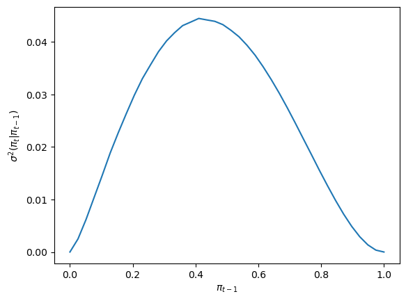
The shape of the conditional variance as a function of \(\pi_{t-1}\) is informative about the behavior of sample paths of \(\{\pi_t\}\).
Notice how the conditional variance approaches \(0\) for \(\pi_{t-1}\) near either \(0\) or \(1\).
The conditional variance is nearly zero only when the agent is almost sure that \(w_t\) is drawn from \(F\), or is almost sure it is drawn from \(G\).