86. Cass-Koopmans Model with Distorting Taxes#
86.1. Overview#
This lecture studies effects of foreseen fiscal and technology shocks on competitive equilibrium prices and quantities in a nonstochastic version of a Cass-Koopmans growth model with features described in this QuantEcon lecture Cass-Koopmans Competitive Equilibrium.
This model is discussed in more detail in chapter 11 of [Ljungqvist and Sargent, 2018].
We use the model as a laboratory to experiment with numerical techniques for approximating equilibria and to display the structure of dynamic models in which decision makers have perfect foresight about future government decisions.
Following a classic paper by Robert E. Hall [Hall, 1971], we augment a nonstochastic version of the Cass-Koopmans optimal growth model with a government that purchases a stream of goods and that finances its purchases with an sequences of several distorting flat-rate taxes.
Distorting taxes prevent a competitive equilibrium allocation from solving a planning problem.
Therefore, to compute an equilibrium allocation and price system, we solve a system of nonlinear difference equations consisting of the first-order conditions for decision makers and the other equilibrium conditions.
We present two ways to approximate an equilibrium:
The first is a shooting algorithm like the one that we deployed in Cass-Koopmans Competitive Equilibrium.
The second method is a root-finding algorithm that minimizes residuals from the first-order conditions of the consumer and representative firm.
86.2. The Economy#
86.2.1. Technology#
Feasible allocations satisfy
where
\(g_t\) is government purchases of the time \(t\) good
\(x_t\) is gross investment, and
\(F(k_t, n_t)\) is a linearly homogeneous production function with positive and decreasing marginal products of capital \(k_t\) and labor \(n_t\).
Physical capital evolves according to
where \(\delta \in (0, 1)\) is a depreciation rate.
It is sometimes convenient to eliminate \(x_t\) from (86.1) and to represent it as as
86.2.2. Components of a competitive equilibrium#
All trades occurring at time \(0\).
The representative household owns capital, makes investment decisions, and rents capital and labor to a representative production firm.
The representative firm uses capital and labor to produce goods with the production function \(F(k_t, n_t)\).
A price system is a triple of sequences \(\{q_t, \eta_t, w_t\}_{t=0}^\infty\), where
\(q_t\) is the time \(0\) pretax price of one unit of investment or consumption at time \(t\) (\(x_t\) or \(c_t\)),
\(\eta_t\) is the pretax price at time \(t\) that the household receives from the firm for renting capital at time \(t\), and
\(w_t\) is the pretax price at time \(t\) that the household receives for renting labor to the firm at time \(t\).
The prices \(w_t\) and \(\eta_t\) are expressed in terms of time \(t\) goods, while \(q_t\) is expressed in terms of a numeraire at time \(0\), as in Cass-Koopmans Competitive Equilibrium.
The presence of a government distinguishes this lecture from Cass-Koopmans Competitive Equilibrium.
Government purchases of goods at time \(t\) are \(g_t \geq 0\).
A government expenditure plan is a sequence \(g = \{g_t\}_{t=0}^\infty\).
A government tax plan is a \(4\)-tuple of sequences \(\{\tau_{ct}, \tau_{kt}, \tau_{nt}, \tau_{ht}\}_{t=0}^\infty\), where
\(\tau_{ct}\) is a tax rate on consumption at time \(t\),
\(\tau_{kt}\) is a tax rate on rentals of capital at time \(t\),
\(\tau_{nt}\) is a tax rate on wage earnings at time \(t\), and
\(\tau_{ht}\) is a lump sum tax on a consumer at time \(t\).
Because lump-sum taxes \(\tau_{ht}\) are available, the government actually should not use any distorting taxes.
Nevertheless, we include all of these taxes because, like [Hall, 1971], they allow us to analyze how various taxes distort production and consumption decisions.
In the experiment section, we shall see how variations in government tax plan affect the transition path and equilibrium.
86.2.3. Representative Household#
A representative household has preferences over nonnegative streams of a single consumption good \(c_t\) and leisure \(1-n_t\) that are ordered by:
where
\(U\) is strictly increasing in \(c_t\), twice continuously differentiable, and strictly concave with \(c_t \geq 0\) and \(n_t \in [0, 1]\).
The representative hßousehold maximizes (86.2) subject to the single budget constraint:
Here we have assumed that the government gives a depreciation allowance \(\delta k_t\) from the gross rentals on capital \(\eta_t k_t\) and so collects taxes \(\tau_{kt} (\eta_t - \delta) k_t\) on rentals from capital.
86.2.4. Government#
Government plans \(\{ g_t \}_{t=0}^\infty\) for government purchases and taxes \(\{\tau_{ct}, \tau_{kt}, \tau_{nt}, \tau_{ht}\}_{t=0}^\infty\) must respect the budget constraint
Given a budget-feasible government policy \(\{g_t\}_{t=0}^\infty\) and \(\{\tau_{ct}, \tau_{kt}, \tau_{nt}, \tau_{ht}\}_{t=0}^\infty\) subject to (86.4),
Household chooses \(\{c_t\}_{t=0}^\infty\), \(\{n_t\}_{t=0}^\infty\), and \(\{k_{t+1}\}_{t=0}^\infty\) to maximize utility(86.2) subject to budget constraint(86.3), and
Firm chooses sequences of capital \(\{k_t\}_{t=0}^\infty\) and \(\{n_t\}_{t=0}^\infty\) to maximize profits
(86.5)#\[ \sum_{t=0}^\infty q_t [F(k_t, n_t) - \eta_t k_t - w_t n_t] \]A feasible allocation is a sequence \(\{c_t, x_t, n_t, k_t\}_{t=0}^\infty\) that satisfies feasibility condition (86.1).
86.3. Equilibrium#
Definition 86.1
A competitive equilibrium with distorting taxes is a budget-feasible government policy, a feasible allocation, and a price system for which, given the price system and the government policy, the allocation solves the household’s problem and the firm’s problem.
86.4. No-arbitrage Condition#
A no-arbitrage argument implies a restriction on prices and tax rates across time.
By rearranging (86.3) and group \(k_t\) at the same \(t\), we can get
The household inherits a given \(k_0\) that it takes as initial condition and is free to choose \(\{ c_t, n_t, k_{t+1} \}_{t=0}^\infty\).
The household’s budget constraint (86.3) must be bounded in equilibrium due to finite resources.
This imposes a restriction on price and tax sequences.
Specifically, for \(t \geq 1\), the terms multiplying \(k_t\) must equal zero.
If they were strictly positive (negative), the household could arbitrarily increase (decrease) the right-hand side of (86.3) by selecting an arbitrarily large positive (negative) \(k_t\), leading to unbounded profit or arbitrage opportunities:
For strictly positive terms, the household could purchase large capital stocks \(k_t\) and profit from their rental services and undepreciated value.
For strictly negative terms, the household could engage in “short selling” synthetic units of capital. Both cases would make (86.3) unbounded.
Hence, by setting the terms multiplying \(k_t\) to \(0\) we have the non-arbitrage condition:
Moreover, we have terminal condition:
Zero-profit conditions for the representative firm impose additional restrictions on equilibrium prices and quantities.
The present value of the firm’s profits is
Applying Euler’s theorem on linearly homogeneous functions to \(F(k, n)\), the firm’s present value is:
No-arbitrage (or zero-profit) conditions are:
86.5. Household’s First Order Condition#
Household maximize (86.2) under (86.3).
Let \(U_1 = \frac{\partial U}{\partial c}, U_2 = \frac{\partial U}{\partial (1-n)} = -\frac{\partial U}{\partial n}.\), we can derive FOC from the Lagrangian
First-order necessary conditions for the representative household’s problem are
and
Rearranging (86.10) and (86.11), we have
Plugging (86.12) into (86.8) and replacing \(q_t\), we get terminal condition
86.6. Computing Equilibria#
To compute an equilibrium, we seek a price system \(\{q_t, \eta_t, w_t\}\), a budget feasible government policy \(\{g_t, \tau_t\} \equiv \{g_t, \tau_{ct}, \tau_{nt}, \tau_{kt}, \tau_{ht}\}\), and an allocation \(\{c_t, n_t, k_{t+1}\}\) that solve a system of nonlinear difference equations consisting of
86.7. Python Code#
We require the following imports
import numpy as np
from scipy.optimize import root
import matplotlib.pyplot as plt
from collections import namedtuple
from mpmath import mp, mpf
from warnings import warn

# Set the precision
mp.dps = 40
mp.pretty = True
We use the mpmath library to perform high-precision arithmetic in the shooting algorithm in cases where the solution diverges due to numerical instability.
Note
In the functions below, we include routines to handle the growth component, which will be discussed further in the section Exogenous growth.
We include them here to avoid code duplication.
We set the following parameters
# Create a namedtuple to store the model parameters
Model = namedtuple("Model",
            ["β", "γ", "δ", "α", "A"])

def create_model(β=0.95, # discount factor
                 γ=2.0,  # relative risk aversion coefficient
                 δ=0.2,  # depreciation rate
                 α=0.33, # capital share
                 A=1.0   # TFP
                 ):
    """Create a model instance."""
    return Model(β=β, γ=γ, δ=δ, α=α, A=A)

model = create_model()

# Total number of periods
S = 100
86.7.1. Inelastic Labor Supply#
In this lecture, we consider the special case where \(U(c, 1-n) = u(c)\) and \(f(k) := F(k, 1)\).
We rewrite (86.1) with \(f(k) := F(k, 1)\),
def next_k(k_t, g_t, c_t, model, μ_t=1):
    """
    Capital next period: k_{t+1} = f(k_t) + (1 - δ) * k_t - c_t - g_t
    with optional growth adjustment: k_{t+1} = (f(k_t) + (1 - δ) * k_t - c_t - g_t) / μ_{t+1}
    """
    return (f(k_t, model) + (1 - model.δ) * k_t - g_t - c_t) / μ_t
By the properties of a linearly homogeneous production function, we have \(F_k(k, n) = f'(k)\) and \(F_n(k, 1) = f(k, 1) - f'(k)k\).
Substituting (86.12), (86.9), and (86.15) into (86.7), we obtain the Euler equation
This can be simplified to:
Equation (86.17) will appear prominently in our equilibrium computation algorithms.
86.7.2. Steady state#
Tax rates and government expenditures act as forcing functions for difference equations (86.15) and (86.17).
Define \(z_t = [g_t, \tau_{kt}, \tau_{ct}]'\).
Represent the second-order difference equation as:
We assume that a government policy reaches a steady state such that \(\lim_{t \to \infty} z_t = \bar z\) and that the steady state prevails for \(t > T\).
The terminal steady-state capital stock \(\bar{k}\) satisfies:
From difference equation (86.17), we can infer a restriction on the steady-state:
86.7.3. Other equilibrium quantities and prices#
Price:
def compute_q_path(c_path, model, S=100, A_path=None):
    """
    Compute q path: q_t = (β^t * u'(c_t)) / u'(c_0)
    with optional A_path for growth models.
    """
    A = np.ones_like(c_path) if A_path is None else np.asarray(A_path)
    q_path = np.zeros_like(c_path)
    for t in range(S):
        q_path[t] = (model.β ** t *
                         u_prime(c_path[t], model, A[t])) / u_prime(c_path[0], model, A[0])
    return q_path
Capital rental rate
def compute_η_path(k_path, model, S=100, A_path=None):
    """
    Compute η path: η_t = f'(k_t)
    with optional A_path for growth models.
    """
    A = np.ones_like(k_path) if A_path is None else np.asarray(A_path)
    η_path = np.zeros_like(k_path)
    for t in range(S):
        η_path[t] = f_prime(k_path[t], model, A[t])
    return η_path
Labor rental rate:
def compute_w_path(k_path, η_path, model, S=100, A_path=None):
    """
    Compute w path: w_t = f(k_t) - k_t * f'(k_t)
    with optional A_path for growth models.
    """
    A = np.ones_like(k_path) if A_path is None else np.asarray(A_path)
    w_path = np.zeros_like(k_path)
    for t in range(S):
        w_path[t] = f(k_path[t], model, A[t]) - k_path[t] * η_path[t]
    return w_path
Gross one-period return on capital:
def compute_R_bar(τ_ct, τ_ctp1, τ_ktp1, k_tp1, model):
    """
    Gross one-period return on capital:
    R_bar = [(1 + τ_c_t) / (1 + τ_c_{t+1})]
        * { [1 - τ_k_{t+1}] * [f'(k_{t+1}) - δ] + 1 }
    """
    return ((1 + τ_ct) / (1 + τ_ctp1)) * (
        (1 - τ_ktp1) * (f_prime(k_tp1, model) - model.δ) + 1)
def compute_R_bar_path(shocks, k_path, model, S=100):
    """
    Compute R_bar path over time.
    """
    R_bar_path = np.zeros(S + 1)
    for t in range(S):
        R_bar_path[t] = compute_R_bar(
            shocks['τ_c'][t], shocks['τ_c'][t + 1], shocks['τ_k'][t + 1],
            k_path[t + 1], model)
    R_bar_path[S] = R_bar_path[S - 1]
    return R_bar_path
One-period discount factor:
Net one-period rate of interest:
By (86.22) and \(r_{t, t+1} = - \ln(\frac{q_{t+1}}{q_t})\), we have
Then by (86.23), we have
Rearranging the above equation, we have
def compute_rts_path(q_path, S, t):
    """
    Compute r path:
    r_t,t+s = - (1/s) * ln(q_{t+s} / q_t)
    """
    s = np.arange(1, S + 1)
    q_path = np.array([float(q) for q in q_path])

    with np.errstate(divide='ignore', invalid='ignore'):
        rts_path = - np.log(q_path[t + s] / q_path[t]) / s
    return rts_path
86.8. Some functional forms#
We assume that the representative household’ period utility has the following CRRA (constant relative risk aversion) form
def u_prime(c, model, A_t=1):
    """
    Marginal utility: u'(c) = c^{-γ}
    with optional technology adjustment: u'(cA) = (cA)^{-γ}
    """
    return (c * A_t) ** (-model.γ)
By substituting (86.21) into (86.17), we obtain
def next_c(c_t, R_bar, model, μ_t=1):
    """
    Consumption next period: c_{t+1} = c_t * (β * R̄)^{1/γ}
    with optional growth adjustment: c_{t+1} = c_t * (β * R_bar)^{1/γ} * μ_{t+1}^{-1}
    """
    return c_t * (model.β * R_bar) ** (1 / model.γ) / μ_t
For the production function we assume a Cobb-Douglas form:
def f(k, model, A=1):
    """
    Production function: f(k) = A * k^{α}
    """
    return A * k ** model.α

def f_prime(k, model, A=1):
    """
    Marginal product of capital: f'(k) = α * A * k^{α - 1}
    """
    return model.α * A * k ** (model.α - 1)
86.9. Computation#
We describe two ways to compute an equilibrium:
a shooting algorithm
a residual-minimization method that focuses on imposing Euler equation (86.17) and the feasibility condition (86.15).
86.9.1. Shooting Algorithm#
This algorithm deploys the following steps.
Solve the equation (86.19) for the terminal steady-state capital \(\bar{k}\) that corresponds to the permanent policy vector \(\bar{z}\).
Select a large time index \(S \gg T\), guess an initial consumption rate \(c_0\), and use the equation (86.15) to solve for \(k_1\).
Use the equation (86.24) to determine \(c_{t+1}\). Then, apply the equation (86.15) to compute \(k_{t+2}\).
Iterate step 3 to compute candidate values \(\hat{k}_t\) for \(t = 1, \dots, S\).
Compute the difference \(\hat{k}_S - \bar{k}\). If \(\left| \hat{k}_S - \bar{k} \right| > \epsilon\) for some small \(\epsilon\), adjust \(c_0\) and repeat steps 2-5.
Adjust \(c_0\) iteratively using the bisection method to find a value that ensures \(\left| \hat{k}_S - \bar{k} \right| < \epsilon\).
The following code implements these steps.
# Steady-state calculation
def steady_states(model, g_ss, τ_k_ss=0.0, μ_ss=None):
    """
    Calculate steady state values for capital and
    consumption with optional A_path for growth models.
    """

    β, δ, α, γ = model.β, model.δ, model.α, model.γ

    A = model.A or 1.0

    # growth‐adjustment in the numerator: μ^γ or 1
    μ_eff = μ_ss**γ if μ_ss is not None else 1.0

    num = δ + (μ_eff/β - 1) / (1 - τ_k_ss)
    k_ss = (num / (α * A)) ** (1 / (α - 1))

    c_ss = (
        A * k_ss**α - δ * k_ss - g_ss
        if μ_ss is None
        else k_ss**α + (1 - δ - μ_ss) * k_ss - g_ss
    )

    return k_ss, c_ss

def shooting_algorithm(
    c0, k0, shocks, S, model, A_path=None):
    """
    Shooting algorithm for given initial c0 and k0
    with optional A_path for growth models.
    """
    # unpack & mpf‐ify shocks, fill μ with ones if missing
    g = np.array(list(map(mpf, shocks['g'])), dtype=object)
    τ_c = np.array(list(map(mpf, shocks['τ_c'])), dtype=object)
    τ_k = np.array(list(map(mpf, shocks['τ_k'])), dtype=object)
    μ = (np.array(list(map(mpf, shocks['μ'])), dtype=object)
              if 'μ' in shocks else np.ones_like(g))
    A = np.ones_like(g) if A_path is None else A_path

    k_path = np.empty(S+1, dtype=object)
    c_path = np.empty(S+1, dtype=object)
    k_path[0], c_path[0] = mpf(k0), mpf(c0)

    for t in range(S):
        k_t, c_t = k_path[t], c_path[t]
        k_tp1 = next_k(k_t, g[t], c_t, model, μ[t+1])
        if k_tp1 < 0:
            return None, None
        k_path[t+1] = k_tp1

        R_bar = compute_R_bar(
            τ_c[t], τ_c[t+1], τ_k[t+1], k_tp1, model
        )
        c_tp1 = next_c(c_t, R_bar, model, μ[t+1])
        if c_tp1 < 0:
            return None, None
        c_path[t+1] = c_tp1

    return k_path, c_path


def bisection_c0(
    c0_guess, k0, shocks, S, model, tol=mpf('1e-6'),
    max_iter=1000, verbose=False, A_path=None):
    """
    Bisection method to find initial c0
    """
    # steady‐state uses last shocks (μ=1 if missing)
    g_last    = mpf(shocks['g'][-1])
    τ_k_last  = mpf(shocks['τ_k'][-1])
    μ_last    = mpf(shocks['μ'][-1]) if 'μ' in shocks else mpf('1')
    k_ss_fin, _ = steady_states(model, g_last, τ_k_last, μ_last)

    c0_lo, c0_hi = mpf('0'), f(k_ss_fin, model)
    c0 = mpf(c0_guess)

    for i in range(1, max_iter+1):
        k_path, _ = shooting_algorithm(c0, k0, shocks, S, model, A_path)
        if k_path is None:
            if verbose:
                print(f"[{i}] shoot failed at c0={c0}")
            c0_hi = c0
        else:
            err = k_path[-1] - k_ss_fin
            if verbose and i % 100 == 0:
                print(f"[{i}] c0={c0}, err={err}")
            if abs(err) < tol:
                if verbose:
                    print(f"Converged after {i} iter")
                return c0
            # update bounds in one line
            c0_lo, c0_hi = (c0, c0_hi) if err > 0 else (c0_lo, c0)
        c0 = (c0_lo + c0_hi) / mpf('2')

    warn(f"bisection did not converge after {max_iter} iters; returning c0={c0}")
    return c0


def run_shooting(
    shocks, S, model, A_path=None,
    c0_finder=bisection_c0, shooter=shooting_algorithm):
    """
    Compute initial SS, find c0, and return [k,c] paths
    with optional A_path for growth models.
    """
    # initial SS at t=0 (μ=1 if missing)
    g0    = mpf(shocks['g'][0])
    τ_k0  = mpf(shocks['τ_k'][0])
    μ0    = mpf(shocks['μ'][0]) if 'μ' in shocks else mpf('1')
    k0, c0 = steady_states(model, g0, τ_k0, μ0)

    optimal_c0 = c0_finder(c0, k0, shocks, S, model, A_path=A_path)
    print(f"Model: {model}\nOptimal initial consumption c0 = {mpf(optimal_c0)}")

    k_path, c_path = shooter(optimal_c0, k0, shocks, S, model, A_path)
    return np.column_stack([k_path, c_path])
86.9.2. Experiments#
Let’s run some experiments.
A foreseen once-and-for-all increase in \(g\) from 0.2 to 0.4 occurring in period 10,
A foreseen once-and-for-all increase in \(\tau_c\) from 0.0 to 0.2 occurring in period 10,
A foreseen once-and-for-all increase in \(\tau_k\) from 0.0 to 0.2 occurring in period 10, and
A foreseen one-time increase in \(g\) from 0.2 to 0.4 in period 10, after which \(g\) reverts to 0.2 permanently.
To start, we prepare sequences that we’ll used to initialize our iterative algorithm.
We will start from an initial steady state and apply shocks at an the indicated time.
def plot_results(
    solution, k_ss, c_ss, shocks, shock_param, axes, model,
    A_path=None, label='', linestyle='-', T=40):
    """
    Plot simulation results (k, c, R, η, and a policy shock)
    with optional A_path for growth models.
    """
    k_path = solution[:, 0]
    c_path = solution[:, 1]
    T = min(T, k_path.size)

    # handle growth parameters
    μ0 = shocks['μ'][0] if 'μ' in shocks else 1.0
    A0 = A_path[0] if A_path is not None else (model.A or 1.0)

    # steady‐state lines
    R_bar_ss = (1 / model.β) * (μ0**model.γ)
    η_ss     = model.α * A0 * k_ss**(model.α - 1)

    # plot k
    axes[0].plot(k_path[:T], linestyle=linestyle, label=label)
    axes[0].axhline(k_ss, linestyle='--', color='black')
    axes[0].set_title('k')

    # plot c
    axes[1].plot(c_path[:T], linestyle=linestyle, label=label)
    axes[1].axhline(c_ss, linestyle='--', color='black')
    axes[1].set_title('c')

    # plot R bar
    S_full    = k_path.size - 1
    R_bar_path = compute_R_bar_path(shocks, k_path, model, S_full)
    axes[2].plot(R_bar_path[:T], linestyle=linestyle, label=label)
    axes[2].axhline(R_bar_ss, linestyle='--', color='black')
    axes[2].set_title(r'$\bar{R}$')

    # plot η
    η_path = compute_η_path(k_path, model, S_full)
    axes[3].plot(η_path[:T], linestyle=linestyle, label=label)
    axes[3].axhline(η_ss, linestyle='--', color='black')
    axes[3].set_title(r'$\eta$')

    # plot shock
    shock_series = np.array(shocks[shock_param], dtype=object)
    axes[4].plot(shock_series[:T], linestyle=linestyle, label=label)
    axes[4].axhline(shock_series[0], linestyle='--', color='black')
    axes[4].set_title(rf'${shock_param}$')

    if label:
        for ax in axes[:5]:
            ax.legend()
Experiment 1: Foreseen once-and-for-all increase in \(g\) from 0.2 to 0.4 in period 10
The figure below shows consequences of a foreseen permanent increase in \(g\) at \(t = T = 10\) that is financed by an increase in lump-sum taxes
# Define shocks as a dictionary
shocks = {
    'g': np.concatenate(
        (np.repeat(0.2, 10), np.repeat(0.4, S - 9))
    ),
    'τ_c': np.repeat(0.0, S + 1),
    'τ_k': np.repeat(0.0, S + 1)
}

k_ss_initial, c_ss_initial = steady_states(model,
                                           shocks['g'][0],
                                           shocks['τ_k'][0])

print(f"Steady-state capital: {k_ss_initial:.4f}")
print(f"Steady-state consumption: {c_ss_initial:.4f}")

solution = run_shooting(shocks, S, model)

fig, axes = plt.subplots(2, 3, figsize=(10, 8))
axes = axes.flatten()

plot_results(solution, k_ss_initial,
             c_ss_initial, shocks, 'g', axes, model, T=40)

for ax in axes[5:]:
    fig.delaxes(ax)

plt.tight_layout()
plt.show()
Steady-state capital: 1.4900
Steady-state consumption: 0.6426
Model: Model(β=0.95, γ=2.0, δ=0.2, α=0.33, A=1.0)
Optimal initial consumption c0 = 0.6092419528879239645312185699727132533517
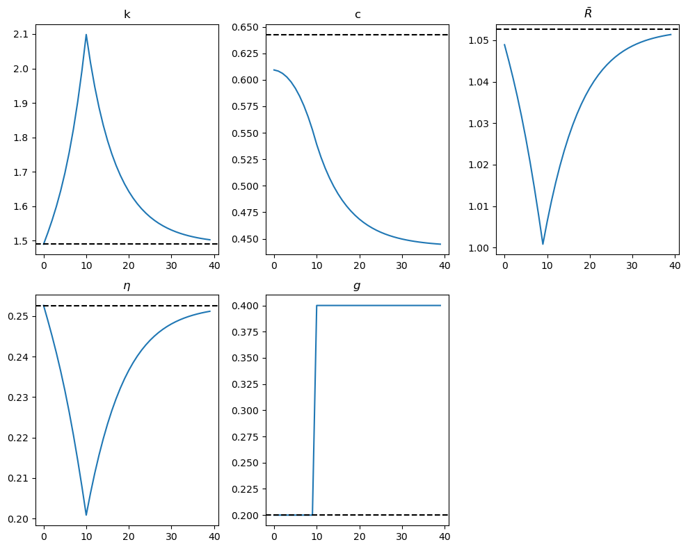
The above figures indicate that an equilibrium consumption smoothing mechanism is at work, driven by the representative consumer’s preference for smooth consumption paths coming from the curvature of its one-period utility function.
The steady-state value of the capital stock remains unaffected:
This follows from the fact that \(g\) disappears from the steady state version of the Euler equation ((86.19)).
Consumption begins to decline gradually before time \(T\) due to increased government consumption:
Households reduce consumption to offset government spending, which is financed through increased lump-sum taxes.
The competitive economy signals households to consume less through an increase in the stream of lump-sum taxes.
Households, caring about the present value rather than the timing of taxes, experience an adverse wealth effect on consumption, leading to an immediate response.
Capital gradually accumulates between time \(0\) and \(T\) due to increased savings and reduces gradually after time \(T\):
This temporal variation in capital stock smooths consumption over time, driven by the representative consumer’s consumption-smoothing motive.
Let’s collect the procedures used above into a function that runs the solver and draws plots for a given experiment
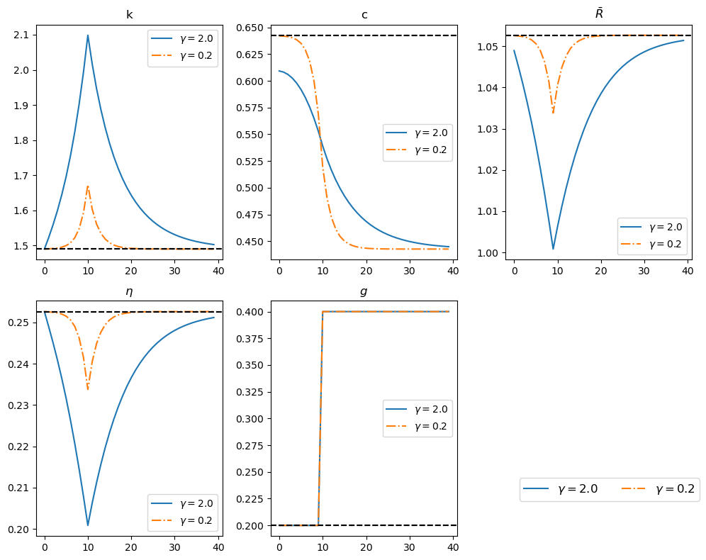
The following figure compares responses to a foreseen increase in \(g\) at \(t = 10\) for two economies:
our original economy with \(\gamma = 2\), shown in the solid line, and
an otherwise identical economy with \(\gamma = 0.2\).
This comparison interest us because the utility curvature parameter \(\gamma\) governs the household’s willingness to substitute consumption over time, and thus it preferences about smoothness of consumption paths over time.
# Solve the model using shooting
solution = run_shooting(shocks, S, model)

# Compute the initial steady states
k_ss_initial, c_ss_initial = steady_states(model,
                                           shocks['g'][0],
                                           shocks['τ_k'][0])

# Plot the solution for γ=2
fig, axes = plt.subplots(2, 3, figsize=(10, 8))
axes = axes.flatten()

label = fr"$\gamma = {model.γ}$"
plot_results(solution, k_ss_initial, c_ss_initial,
             shocks, 'g', axes, model, label=label,
             T=40)

# Solve and plot the result for γ=0.2
model_γ2 = create_model(γ=0.2)
solution = run_shooting(shocks, S, model_γ2)

plot_results(solution, k_ss_initial, c_ss_initial,
             shocks, 'g', axes, model_γ2,
             label=fr"$\gamma = {model_γ2.γ}$",
             linestyle='-.', T=40)

handles, labels = axes[0].get_legend_handles_labels()
fig.legend(handles, labels, loc='lower right',
           ncol=3, fontsize=14, bbox_to_anchor=(1, 0.1))

for ax in axes[5:]:
    fig.delaxes(ax)

plt.tight_layout()
plt.show()
Model: Model(β=0.95, γ=2.0, δ=0.2, α=0.33, A=1.0)
Optimal initial consumption c0 = 0.6092419528879239645312185699727132533517
Model: Model(β=0.95, γ=0.2, δ=0.2, α=0.33, A=1.0)
Optimal initial consumption c0 = 0.6420330412987902926414768724607623681745
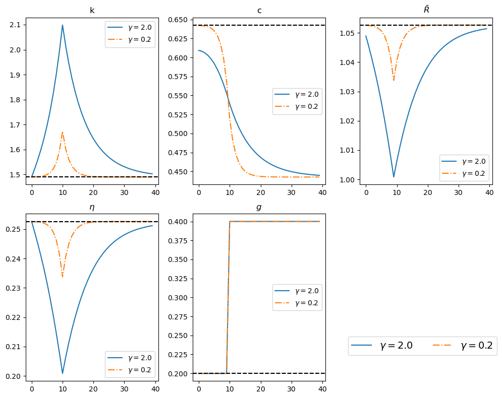
The outcomes indicate that lowering \(\gamma\) affects both the consumption and capital stock paths because - it increases the representative consumer’s willingness to substitute consumption across time:
Consumption path:
When \(\gamma = 0.2\), consumption becomes less smooth compared to \(\gamma = 2\).
For \(\gamma = 0.2\), consumption mirrors the government expenditure path more closely, staying higher until \(t = 10\).
Capital stock path:
With \(\gamma = 0.2\), there are smaller build-ups and drawdowns of capital stock.
There are also smaller fluctuations in \(\bar{R}\) and \(\eta\).
Let’s write another function that runs the solver and draws plots for these two experiments
Now we plot other equilibrium quantities:
def plot_prices(solution, c_ss, shock_param, axes,
                model, label='', linestyle='-', T=40):
    """
    Compares and plots prices
    """
    α, β, δ, γ, A = model.α, model.β, model.δ, model.γ, model.A

    k_path = solution[:, 0]
    c_path = solution[:, 1]

    # Plot for c
    axes[0].plot(c_path[:T], linestyle=linestyle, label=label)
    axes[0].axhline(c_ss, linestyle='--', color='black')
    axes[0].set_title('c')

    # Plot for q
    q_path = compute_q_path(c_path, model, S=S)
    axes[1].plot(q_path[:T], linestyle=linestyle, label=label)
    axes[1].plot(β**np.arange(T), linestyle='--', color='black')
    axes[1].set_title('q')

    # Plot for r_{t,t+1}
    R_bar_path = compute_R_bar_path(shocks, k_path, model, S)
    axes[2].plot(R_bar_path[:T] - 1, linestyle=linestyle, label=label)
    axes[2].axhline(1 / β - 1, linestyle='--', color='black')
    axes[2].set_title('$r_{t,t+1}$')

    # Plot for r_{t,t+s}
    for style, s in zip(['-', '-.', '--'], [0, 10, 60]):
        rts_path = compute_rts_path(q_path, T, s)
        axes[3].plot(rts_path, linestyle=style,
                     color='black' if style == '--' else None,
                     label=f'$t={s}$')
        axes[3].set_xlabel('s')
        axes[3].set_title('$r_{t,t+s}$')

    # Plot for g
    axes[4].plot(shocks[shock_param][:T], linestyle=linestyle, label=label)
    axes[4].axhline(shocks[shock_param][0], linestyle='--', color='black')
    axes[4].set_title(shock_param)
For \(\gamma = 2\) again, the next figure describes the response of \(q_t\) and the term structure of interest rates to a foreseen increase in \(g_t\) at \(t = 10\)
solution = run_shooting(shocks, S, model)

fig, axes = plt.subplots(2, 3, figsize=(10, 8))
axes = axes.flatten()

plot_prices(solution, c_ss_initial, 'g', axes, model, T=40)

for ax in axes[5:]:
    fig.delaxes(ax)

handles, labels = axes[3].get_legend_handles_labels()
fig.legend(handles, labels, title=r"$r_{t,t+s}$ with ", loc='lower right',
           ncol=3, fontsize=10, bbox_to_anchor=(1, 0.1))
plt.tight_layout()
plt.show()
Model: Model(β=0.95, γ=2.0, δ=0.2, α=0.33, A=1.0)
Optimal initial consumption c0 = 0.6092419528879239645312185699727132533517
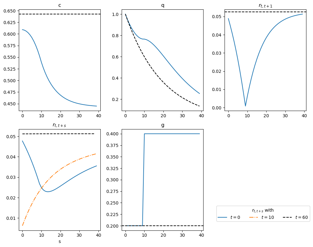
The second panel on the top compares \(q_t\) for the initial steady state with \(q_t\) after the increase in \(g\) is foreseen at \(t = 0\), while the third panel compares the implied short rate \(r_t\).
The fourth panel shows the term structure of interest rates at \(t=0\), \(t=10\), and \(t=60\).
Notice that, by \(t = 60\), the system has converged to the new steady state, and the term structure of interest rates becomes flat.
At \(t = 10\), the term structure of interest rates is upward sloping.
This upward slope reflects the expected increase in the rate of growth of consumption over time, as shown in the consumption panel.
At \(t = 0\), the term structure of interest rates exhibits a “U-shaped” pattern:
It declines until maturity at \(s = 10\).
After \(s = 10\), it increases for longer maturities.
This pattern aligns with the pattern of consumption growth in the first two figures, which declines at an increasing rate until \(t = 10\) and then declines at a decreasing rate afterward.
Experiment 2: Foreseen once-and-for-all increase in \(\tau_c\) from 0.0 to 0.2 in period 10
With an inelastic labor supply, the Euler equation (86.16) and the other equilibrium conditions show that
constant consumption taxes do not distort decisions, but
anticipated changes in them do.
Indeed, (86.16) or (86.17) indicates that a foreseen in- crease in \(\tau_{ct}\) (i.e., a decrease in \((1+\tau_{ct})\) \((1+\tau_{ct+1})\)) operates like an increase in \(\tau_{kt}\).
The following figure portrays the response to a foreseen increase in the consumption tax \(\tau_c\).
shocks = {
    'g': np.repeat(0.2, S + 1),
    'τ_c': np.concatenate((np.repeat(0.0, 10), np.repeat(0.2, S - 9))),
    'τ_k': np.repeat(0.0, S + 1)
}

experiment_model(shocks, S, model,
                 solver=run_shooting,
                 plot_func=plot_results,
                 policy_shock='τ_c')
Steady-state capital: 1.4900
Steady-state consumption: 0.6426
----------------------------------------------------------------
Model: Model(β=0.95, γ=2.0, δ=0.2, α=0.33, A=1.0)
Optimal initial consumption c0 = 0.6492795614681543372301864705195788398396
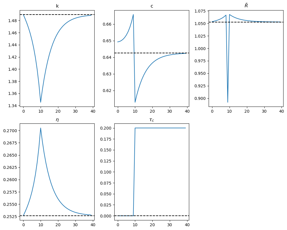
Evidently all variables in the figures above eventually return to their initial steady-state values.
The anticipated increase in \(\tau_{ct}\) leads to variations in consumption and capital stock across time:
At \(t = 0\):
Anticipation of the increase in \(\tau_c\) causes an immediate jump in consumption.
This is followed by a consumption binge that sends the capital stock downward until \(t = T = 10\).
Between \(t = 0\) and \(t = T = 10\):
The decline in the capital stock raises \(\bar{R}\) over time.
The equilibrium conditions require the growth rate of consumption to rise until \(t = T\).
At \(t = T = 10\):
The jump in \(\tau_c\) depresses \(\bar{R}\) below \(1\), causing a sharp drop in consumption.
After \(T = 10\):
The effects of anticipated distortion are over, and the economy gradually adjusts to the lower capital stock.
Capital must now rise, requiring austerity –consumption plummets after \(t = T\), indicated by lower levels of consumption.
The interest rate gradually declines, and consumption grows at a diminishing rate along the path to the terminal steady-state.
Experiment 3: Foreseen once-and-for-all increase in \(\tau_k\) from 0.0 to 0.2 in period 10
For the two \(\gamma\) values 2 and 0.2, the next figure shows the response to a foreseen permanent jump in \(\tau_{kt}\) at \(t = T = 10\).
shocks = {
    'g': np.repeat(0.2, S + 1),
    'τ_c': np.repeat(0.0, S + 1),
    'τ_k': np.concatenate((np.repeat(0.0, 10), np.repeat(0.2, S - 9)))
}

experiment_two_models(shocks, S, model, model_γ2,
                solver=run_shooting,
                 plot_func=plot_results,
                 policy_shock='τ_k')
Model 1 (γ=2.0): steady state k=1.4900, c=0.6426
Model 2 (γ=0.2): steady state k=1.4900, c=0.6426
----------------------------------------------------------------
Model: Model(β=0.95, γ=2.0, δ=0.2, α=0.33, A=1.0)
Optimal initial consumption c0 = 0.6448856400318608460996300822707014890199
Model: Model(β=0.95, γ=0.2, δ=0.2, α=0.33, A=1.0)
Optimal initial consumption c0 = 0.6428407772240506727464152695921513767415
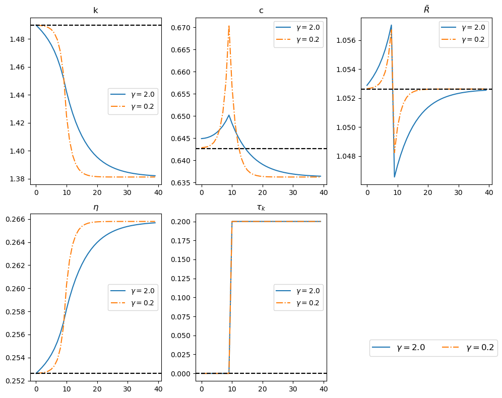
The path of government expenditures remains fixed
the increase in \(\tau_{kt}\) is offset by a reduction in the present value of lump-sum taxes to keep the budget balanced.
The figure shows that:
Anticipation of the increase in \(\tau_{kt}\) leads to immediate decline in capital stock due to increased current consumption and a growing consumption flow.
\(\bar{R}\) starts rising at \(t = 0\) and peaks at \(t = 9\), and at \(t = 10\), \(\bar{R}\) drops sharply due to the tax change.
Variations in \(\bar{R}\) align with the impact of the tax increase at \(t = 10\) on consumption across time.
Transition dynamics push \(k_t\) (capital stock) toward a new, lower steady-state level. In the new steady state:
Consumption is lower due to reduced output from the lower capital stock.
Smoother consumption paths occur when \(\gamma = 2\) than when \(\gamma = 0.2\).
So far we have explored consequences of foreseen once-and-for-all changes in government policy. Next we describe some experiments in which there is a foreseen one-time change in a policy variable (a “pulse”).
Experiment 4: Foreseen one-time increase in \(g\) from 0.2 to 0.4 in period 10, after which \(g\) returns to 0.2 forever
g_path = np.repeat(0.2, S + 1)
g_path[10] = 0.4

shocks = {
    'g': g_path,
    'τ_c': np.repeat(0.0, S + 1),
    'τ_k': np.repeat(0.0, S + 1)
}

experiment_model(shocks, S, model,
                 solver=run_shooting,
                 plot_func=plot_results,
                 policy_shock='g')
Steady-state capital: 1.4900
Steady-state consumption: 0.6426
----------------------------------------------------------------
Model: Model(β=0.95, γ=2.0, δ=0.2, α=0.33, A=1.0)
Optimal initial consumption c0 = 0.6378298012463969247674771825320030214755

The figure indicates how:
Consumption:
Drops immediately upon announcement of the policy and continues to decline over time in anticipation of the one-time surge in \(g\).
After the shock at \(t = 10\), consumption begins to recover, rising at a diminishing rate toward its steady-state value.
Capital and \(\bar{R}\):
Before \(t = 10\), capital accumulates as interest rate changes induce households to prepare for the anticipated increase in government spending.
At \(t = 10\), the capital stock sharply decreases as the government consumes part of it.
\(\bar{R}\) jumps above its steady-state value due to the capital reduction and then gradually declines toward its steady-state level.
86.9.3. Method 2: Residual Minimization#
The second method involves minimizing residuals (i.e., deviations from equalities) of the following equations:
The Euler equation (86.17):
\[ 1 = \beta \left(\frac{c_{t+1}}{c_t}\right)^{-\gamma} \frac{(1+\tau_{ct})}{(1+\tau_{ct+1})} \left[(1 - \tau_{kt+1})(\alpha A k_{t+1}^{\alpha-1} - \delta) + 1 \right] \]The feasibility condition (86.15):
\[ k_{t+1} = A k_{t}^{\alpha} + (1 - \delta) k_t - g_t - c_t. \]
# Euler's equation and feasibility condition
def euler_residual(c_t, c_tp1, τ_c_t, τ_c_tp1, τ_k_tp1, k_tp1, model, μ_tp1=1):
    """
    Computes the residuals for Euler's equation
    with optional growth model parameters μ_tp1.
    """
    R_bar = compute_R_bar(τ_c_t, τ_c_tp1, τ_k_tp1, k_tp1, model)

    c_expected = next_c(c_t, R_bar, model, μ_tp1)

    return c_expected / c_tp1 - 1.0

def feasi_residual(k_t, k_tm1, c_tm1, g_t, model, μ_t=1):
    """
    Computes the residuals for feasibility condition
    with optional growth model parameter μ_t.
    """
    k_t_expected = next_k(k_tm1, g_t, c_tm1, model, μ_t)
    return k_t_expected - k_t
The algorithm proceeds follows:
Find initial steady state \(k_0\) based on the government plan at \(t=0\).
Initialize a sequence of initial guesses \(\{\hat{c}_t, \hat{k}_t\}_{t=0}^{S}\).
Compute residuals \(l_a\) and \(l_k\) for \(t = 0, \dots, S\), as well as \(l_{k_0}\) for \(t = 0\) and \(l_{k_S}\) for \(t = S\):
Compute the Euler equation residual for \(t = 0, \dots, S\) using (86.17):
\[ l_{ta} = \beta u'(c_{t+1}) \frac{(1 + \tau_{ct})}{(1 + \tau_{ct+1})} \left[(1 - \tau_{kt+1})(f'(k_{t+1}) - \delta) + 1 \right] - 1 \]Compute the feasibility condition residual for \(t = 1, \dots, S-1\) using (86.15):
\[ l_{tk} = k_{t+1} - f(k_t) - (1 - \delta)k_t + g_t + c_t \]Compute the residual for the initial condition for \(k_0\) using (86.19) and the initial capital \(k_0\):
\[ l_{k_0} = 1 - \beta \left[ (1 - \tau_{k0}) \left(f'(k_0) - \delta \right) + 1 \right] \]Compute the residual for the terminal condition for \(t = S\) using (86.17) under the assumptions \(c_t = c_{t+1} = c_S\), \(k_t = k_{t+1} = k_S\), \(\tau_{ct} = \tau_{ct+1} = \tau_{c_s}\), and \(\tau_{kt} = \tau_{kt+1} = \tau_{k_s}\):
\[ l_{k_S} = \beta u'(c_S) \frac{(1 + \tau_{c_s})}{(1 + \tau_{c_s})} \left[(1 - \tau_{k_s})(f'(k_S) - \delta) + 1 \right] - 1 \]
Iteratively adjust guesses for \(\{\hat{c}_t, \hat{k}_t\}_{t=0}^{S}\) to minimize residuals \(l_{k_0}\), \(l_{ta}\), \(l_{tk}\), and \(l_{k_S}\) for \(t = 0, \dots, S\).
def compute_residuals(vars_flat, k_init, S, shock_paths, model):
    """
    Compute the residuals for the Euler equation and feasibility condition.
    """
    g, τ_c, τ_k, μ = (shock_paths[key] for key in ('g','τ_c','τ_k','μ'))
    k, c = vars_flat.reshape((S+1, 2)).T
    res = np.empty(2*S+2, dtype=float)

    # boundary condition on initial capital
    res[0] = k[0] - k_init

    # interior Euler and feasibility
    for t in range(S):
        res[2*t + 1] = euler_residual(
            c[t],    c[t+1],
            τ_c[t],  τ_c[t+1],
            τ_k[t+1],k[t+1],
            model, μ[t+1])
        res[2*t + 2] = feasi_residual(
            k[t+1], k[t], c[t],
            g[t],  model,
            μ[t+1])

    # terminal Euler condition at t=S
    res[-1] = euler_residual(
        c[S],   c[S],
        τ_c[S], τ_c[S],
        τ_k[S], k[S],
        model,
        μ[S])

    return res


def run_min(shocks, S, model, A_path=None):
    """
    Solve for the full (k,c) path by root‐finding the residuals.
    """
    shocks['μ'] = shocks['μ'] if 'μ' in shocks else np.ones_like(shocks['g'])

    # compute the steady‐state to serve as both initial capital and guess
    k_ss, c_ss = steady_states(
        model,
        shocks['g'][0],
        shocks['τ_k'][0],
        shocks['μ'][0]  # =1 if no growth
    )

    # initial guess: flat at the steady‐state
    guess = np.column_stack([
        np.full(S+1, k_ss),
        np.full(S+1, c_ss)
    ]).flatten()

    sol = root(
        compute_residuals,
        guess,
        args=(k_ss, S, shocks, model),
        tol=1e-8
    )

    return sol.x.reshape((S+1, 2))
We found that method 2 did not encounter numerical stability issues, so using mp.mpf is not necessary.
We leave as exercises replicating some of our experiments by using the second method.
Exercise 86.1
Replicate the plots of our four experiments using the second method of residual minimization:
A foreseen once-and-for-all increase in \(g\) from 0.2 to 0.4 occurring in period 10,
A foreseen once-and-for-all increase in \(\tau_c\) from 0.0 to 0.2 occurring in period 10,
A foreseen once-and-for-all increase in \(\tau_k\) from 0.0 to 0.2 occurring in period 10, and
A foreseen one-time increase in \(g\) from 0.2 to 0.4 in period 10, after which \(g\) reverts to 0.2 permanently,
Solution
Here is one solution:
Experiment 1: Foreseen once-and-for-all increase in \(g\) from 0.2 to 0.4 in period 10
shocks = {
    'g': np.concatenate((np.repeat(0.2, 10), np.repeat(0.4, S - 9))),
    'τ_c': np.repeat(0.0, S + 1),
    'τ_k': np.repeat(0.0, S + 1)
}

experiment_model(shocks, S, model, solver=run_min,
                 plot_func=plot_results,
                 policy_shock='g')
Steady-state capital: 1.4900
Steady-state consumption: 0.6426
----------------------------------------------------------------
experiment_two_models(shocks, S, model, model_γ2,
                run_min, plot_results, 'g')
Model 1 (γ=2.0): steady state k=1.4900, c=0.6426
Model 2 (γ=0.2): steady state k=1.4900, c=0.6426
----------------------------------------------------------------
solution = run_min(shocks, S, model)

fig, axes = plt.subplots(2, 3, figsize=(10, 8))
axes = axes.flatten()

plot_prices(solution, c_ss_initial, 'g', axes, model, T=40)

for ax in axes[5:]:
    fig.delaxes(ax)

handles, labels = axes[3].get_legend_handles_labels()
fig.legend(handles, labels, title=r"$r_{t,t+s}$ with ", loc='lower right', ncol=3, fontsize=10, bbox_to_anchor=(1, 0.1))
plt.tight_layout()
plt.show()

Experiment 2: Foreseen once-and-for-all increase in \(\tau_c\) from 0.0 to 0.2 in period 10.
shocks = {
    'g': np.repeat(0.2, S + 1),
    'τ_c': np.concatenate((np.repeat(0.0, 10), np.repeat(0.2, S - 9))),
    'τ_k': np.repeat(0.0, S + 1)
}

experiment_model(shocks, S, model, solver=run_min,
                 plot_func=plot_results,
                 policy_shock='τ_c')
Steady-state capital: 1.4900
Steady-state consumption: 0.6426
----------------------------------------------------------------
Experiment 3: Foreseen once-and-for-all increase in \(\tau_k\) from 0.0 to 0.2 in period 10.
shocks = {
    'g': np.repeat(0.2, S + 1),
    'τ_c': np.repeat(0.0, S + 1),
    'τ_k': np.concatenate((np.repeat(0.0, 10), np.repeat(0.2, S - 9)))
}

experiment_two_models(shocks, S, model, model_γ2,
                solver=run_min,
                 plot_func=plot_results,
                 policy_shock='τ_k')
Model 1 (γ=2.0): steady state k=1.4900, c=0.6426
Model 2 (γ=0.2): steady state k=1.4900, c=0.6426
----------------------------------------------------------------
Experiment 4: Foreseen one-time increase in \(g\) from 0.2 to 0.4 in period 10, after which \(g\) returns to 0.2 forever
g_path = np.repeat(0.2, S + 1)
g_path[10] = 0.4

shocks = {
    'g': g_path,
    'τ_c': np.repeat(0.0, S + 1),
    'τ_k': np.repeat(0.0, S + 1)
}

experiment_model(shocks, S, model, solver=run_min,
                 plot_func=plot_results,
                 policy_shock='g')
Steady-state capital: 1.4900
Steady-state consumption: 0.6426
----------------------------------------------------------------
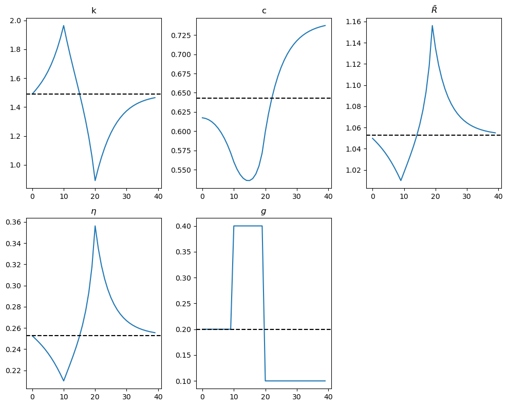
Exercise 86.2
Design a new experiment where the government expenditure \(g\) increases from \(0.2\) to \(0.4\) in period \(10\), and then decreases to \(0.1\) in period \(20\) permanently.
Solution
Here is one solution:
g_path = np.repeat(0.2, S + 1)
g_path[10:20] = 0.4
g_path[20:] = 0.1

shocks = {
    'g': g_path,
    'τ_c': np.repeat(0.0, S + 1),
    'τ_k': np.repeat(0.0, S + 1)
}

experiment_model(shocks, S, model, solver=run_min,
                 plot_func=plot_results,
                 policy_shock='g')
Steady-state capital: 1.4900
Steady-state consumption: 0.6426
----------------------------------------------------------------
86.10. Exogenous growth#
In the previous section, we considered a model without exogenous growth.
We set the term \(A_t\) in the production function to a constant by setting \(A_t = 1\) for all \(t\).
Now we are ready to consider growth.
To incorporate growth, we modify the production function to be
where \(Y_t\) is aggregate output, \(N_t\) is total employment, \(A_t\) is labor-augmenting technical change, and \(F(K, AN)\) is the same linearly homogeneous production function as before.
We assume that \(A_t\) follows the process
and that \(\mu_{t+1}=\bar{\mu}>1\).
# Set the constant A parameter to None
model = create_model(A=None)
def compute_A_path(A0, shocks, S=100):
    """
    Compute A path over time.
    """
    A_path = np.full(S + 1, A0)
    for t in range(1, S + 1):
        A_path[t] = A_path[t-1] * shocks['μ'][t-1]
    return A_path
86.10.1. Inelastic Labor Supply#
By linear homogeneity, the production function can be expressed as
where \(f(k)=F(k,1) = k^\alpha\) and \(k_t=\frac{K_t}{n_tA_t}\), \(y_t=\frac{Y_t}{n_tA_t}\).
\(k_t\) and \(y_t\) are measured per unit of “effective labor” \(A_tn_t\).
We also let \(c_t=\frac{C_t}{A_tn_t}\) and \(g_t=\frac{G_t}{A_tn_t}\), where \(C_t\) and \(G_t\) are total consumption and total government expenditures.
We continue to consider the case of inelastic labor supply.
Based on this, feasibility can be summarized by the following modified version of equation (86.15):
Again, by the properties of a linearly homogeneous production function, we have
Since per capita consumption is now \(c_tA_t\), the counterpart to the Euler equation (86.17) is
\(\bar{R}_{t+1}\) continues to be defined by (86.21), except that now \(k_t\) is capital per effective unit of labor.
Thus, substituting (86.21), (86.27) becomes
Assuming that the household’s utility function is the same as before, we have
Thus, the counterpart to (86.24) is
86.10.2. Steady State#
In a steady state, \(c_{t+1} = c_t\). Then (86.27) becomes
from which we can compute that the steady-state level of capital per unit of effective labor satisfies
and that
The steady-state level of consumption per unit of effective labor can be found using (86.26):
Since the algorithm and plotting routines are the same as before, we include the steady-state calculations and shooting routine in the section Python Code.
86.10.3. Shooting Algorithm#
Now we can apply the shooting algorithm to compute equilibrium. We augment the vector of shock variables by including \(\mu_t\), then proceed as before.
86.10.4. Experiments#
Let’s run some experiments:
A foreseen once-and-for-all increase in \(\mu\) from 1.02 to 1.025 in period 10
An unforeseen once-and-for-all increase in \(\mu\) to 1.025 in period 0
86.10.4.1. Experiment 1: A foreseen increase in \(\mu\) from 1.02 to 1.025 at t=10#
The figures below show the effects of a permanent increase in productivity growth \(\mu\) from 1.02 to 1.025 at t=10.
They now measure \(c\) and \(k\) in effective units of labor.
shocks = {
    'g': np.repeat(0.2, S + 1),
    'τ_c': np.repeat(0.0, S + 1),
    'τ_k': np.repeat(0.0, S + 1),
    'μ': np.concatenate((np.repeat(1.02, 10), np.repeat(1.025, S - 9)))
}

A_path = compute_A_path(1.0, shocks, S)

k_ss_initial, c_ss_initial = steady_states(model,
                                         shocks['g'][0],
                                         shocks['τ_k'][0],
                                         shocks['μ'][0]
                                        )

print(f"Steady-state capital: {k_ss_initial:.4f}")
print(f"Steady-state consumption: {c_ss_initial:.4f}")

# Run the shooting algorithm with the A_path parameter
solution = run_shooting(shocks, S, model, A_path)

fig, axes = plt.subplots(2, 3, figsize=(10, 8))
axes = axes.flatten()

plot_results(solution, k_ss_initial,
             c_ss_initial, shocks, 'μ', axes, model,
             A_path, T=40)

for ax in axes[5:]:
    fig.delaxes(ax)

plt.tight_layout()
plt.show()
Steady-state capital: 1.1812
Steady-state consumption: 0.5966
Model: Model(β=0.95, γ=2.0, δ=0.2, α=0.33, A=None)
Optimal initial consumption c0 = 0.5971184749344462396270918337183607339919
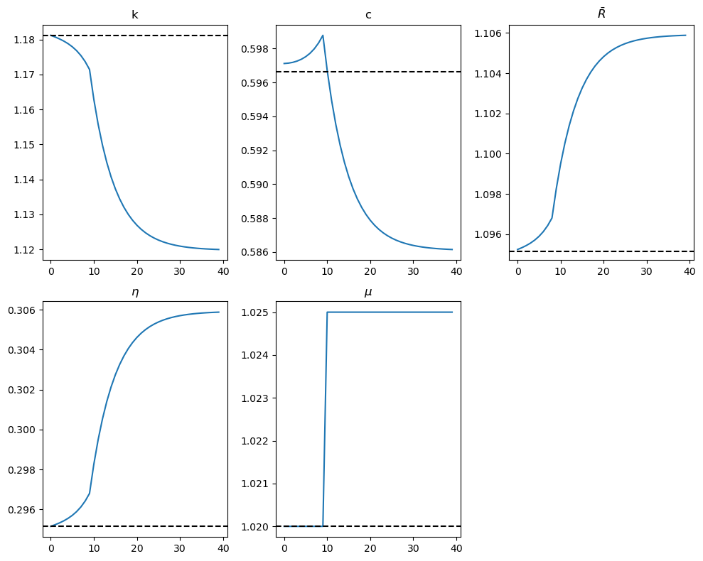
The results in the figures are mainly driven by (86.29) and imply that a permanent increase in \(\mu\) will lead to a decrease in the steady-state value of capital per unit of effective labor.
The figures indicate the following:
As capital becomes more efficient, even with less of it, consumption per capita can be raised.
Consumption smoothing drives an immediate jump in consumption in anticipation of the increase in \(\mu\).
The increased productivity of capital leads to an increase in the gross return \(\bar R\).
Perfect foresight makes the effects of the increase in the growth of capital precede it, with the effect visible at \(t=0\).
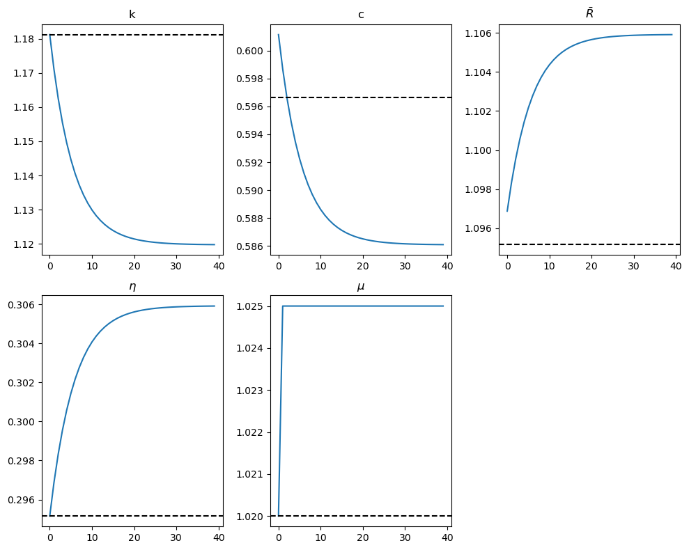
86.10.4.2. Experiment 2: An unforeseen increase in \(\mu\) from 1.02 to 1.025 at t=0#
The figures below show the effects of an immediate jump in \(\mu\) to 1.025 at t=0.
shocks = {
    'g': np.repeat(0.2, S + 1),
    'τ_c': np.repeat(0.0, S + 1),
    'τ_k': np.repeat(0.0, S + 1),
    'μ': np.concatenate((np.repeat(1.02, 1), np.repeat(1.025, S)))
}

A_path = compute_A_path(1.0, shocks, S)

k_ss_initial, c_ss_initial = steady_states(model,
                                           shocks['g'][0],
                                           shocks['τ_k'][0],
                                           shocks['μ'][0]
                                          )

print(f"Steady-state capital: {k_ss_initial:.4f}")
print(f"Steady-state consumption: {c_ss_initial:.4f}")

# Run the shooting algorithm with the A_path parameter
solution = run_shooting(shocks, S, model, A_path)

fig, axes = plt.subplots(2, 3, figsize=(10, 8))
axes = axes.flatten()

plot_results(solution, k_ss_initial,
             c_ss_initial, shocks, 'μ', axes, model, A_path, T=40)

for ax in axes[5:]:
    fig.delaxes(ax)

plt.tight_layout()
plt.show()
Steady-state capital: 1.1812
Steady-state consumption: 0.5966
Model: Model(β=0.95, γ=2.0, δ=0.2, α=0.33, A=None)
Optimal initial consumption c0 = 0.6011494930430641150395883753109588316638
Again, we can collect the procedures used above into a function that runs the solver and draws plots for a given experiment.
def experiment_model(shocks, S, model, A_path, solver, plot_func, policy_shock, T=40):
    """
    Run the shooting algorithm given a model and plot the results.
    """
    k0, c0 = steady_states(model, shocks['g'][0], shocks['τ_k'][0], shocks['μ'][0])

    print(f"Steady-state capital: {k0:.4f}")
    print(f"Steady-state consumption: {c0:.4f}")
    print('-'*64)

    fig, axes = plt.subplots(2, 3, figsize=(10, 8))
    axes = axes.flatten()

    solution = solver(shocks, S, model, A_path)
    plot_func(solution, k0, c0,
              shocks, policy_shock, axes, model, A_path, T=T)

    for ax in axes[5:]:
        fig.delaxes(ax)

    plt.tight_layout()
    plt.show()
shocks = {
    'g': np.repeat(0.2, S + 1),
    'τ_c': np.repeat(0.0, S + 1),
    'τ_k': np.repeat(0.0, S + 1),
    'μ': np.concatenate((np.repeat(1.02, 1), np.repeat(1.025, S)))
}

experiment_model(shocks, S, model, A_path, run_shooting, plot_results, 'μ')
Steady-state capital: 1.1812
Steady-state consumption: 0.5966
----------------------------------------------------------------
Model: Model(β=0.95, γ=2.0, δ=0.2, α=0.33, A=None)
Optimal initial consumption c0 = 0.6011494930430641150395883753109588316638
The figures show that:
The paths of all variables are now smooth due to the absence of feedforward effects.
Capital per effective unit of labor gradually declines to a lower steady-state level.
Consumption per effective unit of labor jumps immediately and then declines smoothly toward its lower steady-state value.
The after-tax gross return \(\bar{R}\) once again co-moves with the consumption growth rate, verifying the Euler equation (86.29).
Exercise 86.3
Replicate the plots of our two experiments using the second method of residual minimization:
A foreseen increase in \(\mu\) from 1.02 to 1.025$ at t=10
An unforeseen increase in \(\mu\) from 1.02 to 1.025$ at t=0
Solution
Here is one solution:
Experiment 1: A foreseen increase in \(\mu\) from 1.02 to 1.025 at \(t=10\)
shocks = {
    'g': np.repeat(0.2, S + 1),
    'τ_c': np.repeat(0.0, S + 1),
    'τ_k': np.repeat(0.0, S + 1),
    'μ': np.concatenate((np.repeat(1.02, 10), np.repeat(1.025, S - 9)))
}

A_path = compute_A_path(1.0, shocks, S)

experiment_model(shocks, S, model, A_path, run_min, plot_results, 'μ')
Steady-state capital: 1.1812
Steady-state consumption: 0.5966
----------------------------------------------------------------
Experiment 2: An unforeseen increase in \(\mu\) from 1.02 to 1.025 at \(t=0\)
shocks = {
    'g': np.repeat(0.2, S + 1),
    'τ_c': np.repeat(0.0, S + 1),
    'τ_k': np.repeat(0.0, S + 1),
    'μ': np.concatenate((np.repeat(1.02, 1), np.repeat(1.025, S)))
}

experiment_model(shocks, S, model, A_path, run_min, plot_results, 'μ')
Steady-state capital: 1.1812
Steady-state consumption: 0.5966
----------------------------------------------------------------
In this this sequel Two-Country Model with Distorting Taxes, we study a two-country version of our one-country model that is closely related to Mendoza and Tesar [1998].