13. Multivariate Normal Distribution#
13.1. Overview#
This lecture describes a workhorse in probability theory, statistics, and economics, namely, the multivariate normal distribution.
In this lecture, you will learn formulas for
the joint distribution of a random vector \(x\) of length \(N\)
marginal distributions for all subvectors of \(x\)
conditional distributions for subvectors of \(x\) conditional on other subvectors of \(x\)
We will use the multivariate normal distribution to formulate some useful models:
a factor analytic model of an intelligence quotient, i.e., IQ
a factor analytic model of two independent inherent abilities, say, mathematical and verbal.
a more general factor analytic model
Principal Components Analysis (PCA) as an approximation to a factor analytic model
time series generated by linear stochastic difference equations
optimal linear filtering theory
13.2. The multivariate normal distribution#
This lecture defines a Python class MultivariateNormal to be used
to generate marginal and conditional distributions associated
with a multivariate normal distribution.
For a multivariate normal distribution it is very convenient that
conditional expectations equal linear least squares projections
conditional distributions are characterized by multivariate linear regressions
We apply our Python class to some examples.
We use the following imports:
import matplotlib.pyplot as plt
import numpy as np
from numba import jit
import statsmodels.api as sm

rng = np.random.default_rng(0)
Assume that an \(N \times 1\) random vector \(z\) has a multivariate normal probability density.
This means that the probability density takes the form
where \(\mu=Ez\) is the mean of the random vector \(z\) and \(\Sigma=E\left(z-\mu\right)\left(z-\mu\right)^\top\) is the covariance matrix of \(z\).
The covariance matrix \(\Sigma\) is symmetric and positive definite.
@jit
def f(z, μ, Σ):
    """
    The density function of multivariate normal distribution.

    Parameters
    ---------------
    z: ndarray(float, dim=2)
        random vector, N by 1
    μ: ndarray(float, dim=1 or 2)
        the mean of z, N by 1
    Σ: ndarray(float, dim=2)
        the covariance matrix of z, N by N
    """

    z = np.atleast_2d(z)
    μ = np.atleast_2d(μ)
    Σ = np.atleast_2d(Σ)

    N = z.size

    temp1 = np.linalg.det(Σ) ** (-1/2)
    temp2 = np.exp(-.5 * (z - μ).T @ np.linalg.inv(Σ) @ (z - μ))

    return (2 * np.pi) ** (-N/2) * temp1 * temp2
For some integer \(k\in \{1,\dots, N-1\}\), partition \(z\) as
where \(z_1\) is an \(\left(N-k\right)\times1\) vector and \(z_2\) is a \(k\times1\) vector.
Let
be corresponding partitions of \(\mu\) and \(\Sigma\).
The marginal distribution of \(z_1\) is
multivariate normal with mean \(\mu_1\) and covariance matrix \(\Sigma_{11}\).
The marginal distribution of \(z_2\) is
multivariate normal with mean \(\mu_2\) and covariance matrix \(\Sigma_{22}\).
The distribution of \(z_1\) conditional on \(z_2\) is
multivariate normal with mean
and covariance matrix
where
is an \(\left(N-k\right) \times k\) matrix of population regression coefficients of the \((N -k) \times 1\) random vector \(z_1 - \mu_1\) on the \(k \times 1\) random vector \(z_2 - \mu_2\).
The following class constructs a multivariate normal distribution instance with two methods.
a method
partitioncomputes \(\beta\), taking \(k\) as an inputa method
cond_distcomputes either the distribution of \(z_1\) conditional on \(z_2\) or the distribution of \(z_2\) conditional on \(z_1\)
class MultivariateNormal:
    """
    Class of multivariate normal distribution.

    Parameters
    ----------
    μ: ndarray(float, dim=1)
        the mean of z, N by 1
    Σ: ndarray(float, dim=2)
        the covariance matrix of z, N by N

    Arguments
    ---------
    μ, Σ:
        see parameters
    μs: list(ndarray(float, dim=1))
        list of mean vectors μ1 and μ2 in order
    Σs: list(list(ndarray(float, dim=2)))
        2 dimensional list of covariance matrices
        Σ11, Σ12, Σ21, Σ22 in order
    βs: list(ndarray(float, dim=1))
        list of regression coefficients β1 and β2 in order
    """

    def __init__(self, μ, Σ):
        "initialization"
        self.μ = np.array(μ)
        self.Σ = np.atleast_2d(Σ)

    def partition(self, k):
        """
        Given k, partition the random vector z into a size k vector z1
        and a size N-k vector z2. Partition the mean vector μ into
        μ1 and μ2, and the covariance matrix Σ into Σ11, Σ12, Σ21, Σ22
        correspondingly. Compute the regression coefficients β1 and β2
        using the partitioned arrays.
        """
        μ = self.μ
        Σ = self.Σ

        self.μs = [μ[:k], μ[k:]]
        self.Σs = [[Σ[:k, :k], Σ[:k, k:]],
                   [Σ[k:, :k], Σ[k:, k:]]]

        self.βs = [self.Σs[0][1] @ np.linalg.inv(self.Σs[1][1]),
                   self.Σs[1][0] @ np.linalg.inv(self.Σs[0][0])]

    def cond_dist(self, ind, z):
        """
        Compute the conditional distribution of z1 given z2, or reversely.
        Argument ind determines whether we compute the conditional
        distribution of z1 (ind=0) or z2 (ind=1).

        Returns
        ---------
        μ_hat: ndarray(float, ndim=1)
            The conditional mean of z1 or z2.
        Σ_hat: ndarray(float, ndim=2)
            The conditional covariance matrix of z1 or z2.
        """
        β = self.βs[ind]
        μs = self.μs
        Σs = self.Σs

        μ_hat = μs[ind] + β @ (z - μs[1-ind])
        Σ_hat = Σs[ind][ind] - β @ Σs[1-ind][1-ind] @ β.T

        return μ_hat, Σ_hat
Let’s put this code to work on a suite of examples.
We begin with a simple bivariate example; after that we’ll turn to a trivariate example.
We’ll compute population moments of some conditional distributions using
our MultivariateNormal class.
For fun we’ll also compute sample analogs of the associated population regressions by generating simulations and then computing linear least squares regressions.
We’ll compare those linear least squares regressions for the simulated data to their population counterparts.
13.3. Bivariate example#
We start with a bivariate normal distribution pinned down by
μ = np.array([.5, 1.])
Σ = np.array([[1., .5], [.5 ,1.]])

# construction of the multivariate normal instance
multi_normal = MultivariateNormal(μ, Σ)
k = 1 # choose partition

# partition and compute regression coefficients
multi_normal.partition(k)
multi_normal.βs[0],multi_normal.βs[1]
(array([[0.5]]), array([[0.5]]))
Let’s illustrate the fact that you can regress anything on anything else.
We have computed everything we need to compute two regression lines, one of \(z_2\) on \(z_1\), the other of \(z_1\) on \(z_2\).
We’ll represent these regressions as
and
where we have the population least squares orthogonality conditions
and
Let’s compute \(a_1, a_2, b_1, b_2\).
β = multi_normal.βs

a1 = μ[0] - β[0]*μ[1]
b1 = β[0]

a2 = μ[1] - β[1]*μ[0]
b2 = β[1]
Let’s print out the intercepts and slopes.
For the regression of \(z_1\) on \(z_2\) we have
print ("a1 = ", a1)
print ("b1 = ", b1)
a1 =  [[0.]]
b1 =  [[0.5]]
For the regression of \(z_2\) on \(z_1\) we have
print ("a2 = ", a2)
print ("b2 = ", b2)
a2 =  [[0.75]]
b2 =  [[0.5]]
Now let’s plot the two regression lines and stare at them.
z2 = np.linspace(-4,4,100)


a1 = np.squeeze(a1)
b1 = np.squeeze(b1)

a2 = np.squeeze(a2)
b2 = np.squeeze(b2)

z1  = b1*z2 + a1


z1h = z2/b2 - a2/b2


fig = plt.figure(figsize=(12,12))
ax = fig.add_subplot(1, 1, 1)
ax.set(xlim=(-4, 4), ylim=(-4, 4))
ax.spines['left'].set_position('center')
ax.spines['bottom'].set_position('zero')
ax.spines['right'].set_color('none')
ax.spines['top'].set_color('none')
ax.xaxis.set_ticks_position('bottom')
ax.yaxis.set_ticks_position('left')
plt.ylabel('$z_1$', loc = 'top')
plt.xlabel('$z_2$,', loc = 'right')
plt.plot(z2,z1, 'r', label = "$z_1$ on $z_2$")
plt.plot(z2,z1h, 'b', label = "$z_2$ on $z_1$")
plt.legend()
plt.show()
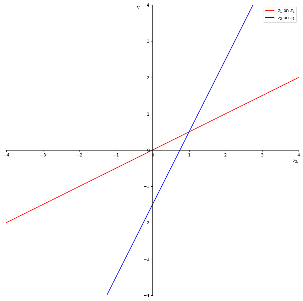
Fig. 13.1 two regressions#
The red line is the expectation of \(z_1\) conditional on \(z_2\).
The intercept and slope of the red line are
print("a1 = ", a1)
print("b1 = ", b1)
a1 =  0.0
b1 =  0.5
The blue line is the expectation of \(z_2\) conditional on \(z_1\).
The intercept and slope of the blue line are
print("-a2/b2 = ", - a2/b2)
print("1/b2 = ", 1/b2)
-a2/b2 =  -1.5
1/b2 =  2.0
We can use these regression lines or our code to compute conditional expectations.
Let’s compute the mean and variance of the distribution of \(z_2\) conditional on \(z_1=5\).
After that we’ll reverse what are on the left and right sides of the regression.
# compute the cond. dist. of z1
ind = 1
z1 = np.array([5.]) # given z1

μ2_hat, Σ2_hat = multi_normal.cond_dist(ind, z1)
print('μ2_hat, Σ2_hat = ', μ2_hat, Σ2_hat)
μ2_hat, Σ2_hat = [3.25] [[0.75]]
Now let’s compute the mean and variance of the distribution of \(z_1\) conditional on \(z_2=5\).
# compute the cond. dist. of z1
ind = 0
z2 = np.array([5.]) # given z2

μ1_hat, Σ1_hat = multi_normal.cond_dist(ind, z2)
print('μ1_hat, Σ1_hat = ', μ1_hat, Σ1_hat)
μ1_hat, Σ1_hat = [2.5] [[0.75]]
Let’s compare the preceding population mean and variance with outcomes from drawing a large sample and then regressing \(z_1 - \mu_1\) on \(z_2 - \mu_2\).
We know that
which can be arranged to
We anticipate that for larger and larger sample sizes, estimated OLS coefficients will converge to \(\beta\) and the estimated variance of \(\epsilon\) will converge to \(\hat{\Sigma}_1\).
n = 1_000_000 # sample size

# simulate multivariate normal random vectors
data = rng.multivariate_normal(μ, Σ, size=n)
z1_data = data[:, 0]
z2_data = data[:, 1]

# OLS regression
μ1, μ2 = multi_normal.μs
results = sm.OLS(z1_data - μ1, z2_data - μ2).fit()
Let’s compare the preceding population \(\beta\) with the OLS sample estimate on \(z_2 - \mu_2\)
multi_normal.βs[0], results.params
(array([[0.5]]), array([0.49918333]))
Let’s compare our population \(\hat{\Sigma}_1\) with the degrees-of-freedom adjusted estimate of the variance of \(\epsilon\)
Σ1_hat, results.resid @ results.resid.T / (n - 1)
(array([[0.75]]), np.float64(0.7489203195072748))
Lastly, let’s compute the estimate of \(\hat{E z_1 | z_2}\) and compare it with \(\hat{\mu}_1\)
μ1_hat, results.predict(z2 - μ2) + μ1
(array([2.5]), array([2.49673331]))
Thus, in each case, for our very large sample size, the sample analogues closely approximate their population counterparts.
A Law of Large Numbers explains why sample analogues approximate population objects.
13.4. Trivariate example#
Let’s apply our code to a trivariate example.
We’ll specify the mean vector and the covariance matrix as follows.
μ = rng.random(3)
C = rng.random((3, 3))
Σ = C @ C.T # positive semi-definite

multi_normal = MultivariateNormal(μ, Σ)
μ, Σ
(array([0.4201905 , 0.04279279, 0.32149359]),
 array([[0.95070417, 0.48194854, 0.38025012],
        [0.48194854, 1.34029754, 0.43476327],
        [0.38025012, 0.43476327, 0.20864566]]))
k = 1
multi_normal.partition(k)
Let’s compute the distribution of \(z_1\) conditional on \(z_{2}=\left[\begin{array}{c} 2\\ 5 \end{array}\right]\).
ind = 0
z2 = np.array([2., 5.])

μ1_hat, Σ1_hat = multi_normal.cond_dist(ind, z2)
n = 1_000_000
data = rng.multivariate_normal(μ, Σ, size=n)
z1_data = data[:, :k]
z2_data = data[:, k:]
μ1, μ2 = multi_normal.μs
results = sm.OLS(z1_data - μ1, z2_data - μ2).fit()
As above, we compare population and sample regression coefficients, the conditional covariance matrix, and the conditional mean vector in that order.
multi_normal.βs[0], results.params
(array([[-0.71459379, 3.311496 ]]), array([-0.71383888, 3.31026328]))
Σ1_hat, results.resid @ results.resid.T / (n - 1)
(array([[0.03590485]]), np.float64(0.035947932906627136))
μ1_hat, results.predict(z2 - μ2) + μ1
(array([14.5144376]), array([14.51014783]))
Once again, sample analogues do a good job of approximating their populations counterparts.
13.5. One dimensional intelligence (IQ)#
Let’s move closer to a real-life example, namely, inferring a one-dimensional measure of intelligence called IQ from a list of test scores.
The \(i\)th test score \(y_i\) equals the sum of an unknown scalar IQ \(\theta\) and a random variable \(w_{i}\).
The distribution of IQ’s for a cross-section of people is a normal random variable described by
We assume that the noises \(\{w_i\}_{i=1}^N\) in the test scores are IID and not correlated with IQ.
We also assume that \(\{w_i\}_{i=1}^{n+1}\) are i.i.d. standard normal:
The following system describes the \((n+1) \times 1\) random vector \(X\) that interests us:
or equivalently,
where \(X = \begin{bmatrix} y \cr \theta \end{bmatrix}\), \(\boldsymbol{1}_{n+1}\) is a vector of \(1\)s of size \(n+1\), and \(D\) is an \(n+1\) by \(n+1\) matrix.
Let’s define a Python function that constructs the mean \(\mu\) and covariance matrix \(\Sigma\) of the random vector \(X\) that we know is governed by a multivariate normal distribution.
As arguments, the function takes the number of tests \(n\), the mean \(\mu_{\theta}\) and the standard deviation \(\sigma_\theta\) of the IQ distribution, and the standard deviation of the randomness in test scores \(\sigma_{y}\).
def construct_moments_IQ(n, μθ, σθ, σy):

    μ_IQ = np.full(n+1, μθ)

    D_IQ = np.zeros((n+1, n+1))
    D_IQ[range(n), range(n)] = σy
    D_IQ[:, n] = σθ

    Σ_IQ = D_IQ @ D_IQ.T

    return μ_IQ, Σ_IQ, D_IQ
Now let’s consider a specific instance of this model.
Assume we have recorded \(50\) test scores and we know that \(\mu_{\theta}=100\), \(\sigma_{\theta}=10\), and \(\sigma_{y}=10\).
We can compute the mean vector and covariance matrix of \(X\) easily
with our construct_moments_IQ function as follows.
n = 50
μθ, σθ, σy = 100., 10., 10.

μ_IQ, Σ_IQ, D_IQ = construct_moments_IQ(n, μθ, σθ, σy)
μ_IQ, Σ_IQ, D_IQ
(array([100., 100., 100., 100., 100., 100., 100., 100., 100., 100., 100.,
        100., 100., 100., 100., 100., 100., 100., 100., 100., 100., 100.,
        100., 100., 100., 100., 100., 100., 100., 100., 100., 100., 100.,
        100., 100., 100., 100., 100., 100., 100., 100., 100., 100., 100.,
        100., 100., 100., 100., 100., 100., 100.]),
 array([[200., 100., 100., ..., 100., 100., 100.],
        [100., 200., 100., ..., 100., 100., 100.],
        [100., 100., 200., ..., 100., 100., 100.],
        ...,
        [100., 100., 100., ..., 200., 100., 100.],
        [100., 100., 100., ..., 100., 200., 100.],
        [100., 100., 100., ..., 100., 100., 100.]], shape=(51, 51)),
 array([[10.,  0.,  0., ...,  0.,  0., 10.],
        [ 0., 10.,  0., ...,  0.,  0., 10.],
        [ 0.,  0., 10., ...,  0.,  0., 10.],
        ...,
        [ 0.,  0.,  0., ..., 10.,  0., 10.],
        [ 0.,  0.,  0., ...,  0., 10., 10.],
        [ 0.,  0.,  0., ...,  0.,  0., 10.]], shape=(51, 51)))
We can now use our MultivariateNormal class to construct an
instance, then partition the mean vector and covariance matrix as we
wish.
We want to regress IQ, the random variable \(\theta\) (what we don’t know), on the vector \(y\) of test scores (what we do know).
We choose k=n so that \(z_{1} = y\) and \(z_{2} = \theta\).
multi_normal_IQ = MultivariateNormal(μ_IQ, Σ_IQ)

k = n
multi_normal_IQ.partition(k)
Using the generator multivariate_normal, we can make one draw of the
random vector from our distribution and then compute the distribution of
\(\theta\) conditional on our test scores.
Let’s do that and then print out some pertinent quantities.
x = rng.multivariate_normal(μ_IQ, Σ_IQ)
y = x[:-1] # test scores
θ = x[-1]  # IQ
# the true value
θ
np.float64(98.2495327983163)
The method cond_dist takes test scores \(y\) as input and returns the
conditional normal distribution of the IQ \(\theta\).
In the following code, ind sets the variables on the right side of the regression.
Given the way we have defined the vector \(X\), we want to set ind=1 in order to make \(\theta\) the left side variable in the
population regression.
ind = 1
multi_normal_IQ.cond_dist(ind, y)
(array([97.20269774]), array([[1.96078431]]))
The first number is the conditional mean \(\hat{\mu}_{\theta}\) and the second is the conditional variance \(\hat{\Sigma}_{\theta}\).
How do additional test scores affect our inferences?
To shed light on this, we compute a sequence of conditional distributions of \(\theta\) by varying the number of test scores in the conditioning set from \(1\) to \(n\).
We’ll make a pretty graph showing how our judgment of the person’s IQ change as more test results come in.
# array for containing moments
μθ_hat_arr = np.empty(n)
Σθ_hat_arr = np.empty(n)

# loop over number of test scores
for i in range(1, n+1):
    # construction of multivariate normal distribution instance
    μ_IQ_i, Σ_IQ_i, D_IQ_i = construct_moments_IQ(i, μθ, σθ, σy)
    multi_normal_IQ_i = MultivariateNormal(μ_IQ_i, Σ_IQ_i)

    # partition and compute conditional distribution
    multi_normal_IQ_i.partition(i)
    scores_i = y[:i]
    μθ_hat_i, Σθ_hat_i = multi_normal_IQ_i.cond_dist(1, scores_i)

    # store the results
    μθ_hat_arr[i-1] = μθ_hat_i[0]
    Σθ_hat_arr[i-1] = Σθ_hat_i[0, 0]

# transform variance to standard deviation
σθ_hat_arr = np.sqrt(Σθ_hat_arr)
μθ_hat_lower = μθ_hat_arr - 1.96 * σθ_hat_arr
μθ_hat_higher = μθ_hat_arr + 1.96 * σθ_hat_arr

plt.hlines(θ, 1, n+1, ls='--', label='true $θ$')
plt.plot(range(1, n+1), μθ_hat_arr, color='b', label=r'$\hat{μ}_{θ}$')
plt.plot(range(1, n+1), μθ_hat_lower, color='b', ls='--')
plt.plot(range(1, n+1), μθ_hat_higher, color='b', ls='--')
plt.fill_between(range(1, n+1), μθ_hat_lower, μθ_hat_higher,
                 color='b', alpha=0.2, label='95%')

plt.xlabel('number of test scores')
plt.ylabel(r'$\hat{θ}$')
plt.legend()

plt.show()
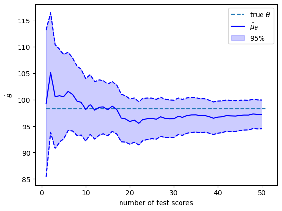
The solid blue line in the plot above shows \(\hat{\mu}_{\theta}\) as a function of the number of test scores that we have recorded and conditioned on.
The blue area shows the span that comes from adding or subtracting \(1.96 \hat{\sigma}_{\theta}\) from \(\hat{\mu}_{\theta}\).
Therefore, \(95\%\) of the probability mass of the conditional distribution falls in this range.
The value of the random \(\theta\) that we drew is shown by the black dotted line.
As more and more test scores come in, our estimate of the person’s \(\theta\) become more and more reliable.
By staring at the changes in the conditional distributions, we see that adding more test scores makes \(\hat{\theta}\) settle down and approach \(\theta\).
Thus, each \(y_{i}\) adds information about \(\theta\).
If we were to drive the number of tests \(n \rightarrow + \infty\), the conditional standard deviation \(\hat{\sigma}_{\theta}\) would converge to \(0\) at rate \(\frac{1}{n^{.5}}\).
13.6. Information as surprise#
By using a different representation, let’s look at things from a different perspective.
We can represent the random vector \(X\) defined above as
where \(C\) is a lower triangular Cholesky factor of \(\Sigma\) so that
and
It follows that
Let \(G=C^{-1}\)
\(G\) is also lower triangular.
We can compute \(\epsilon\) from the formula
This formula confirms that the orthonormal vector \(\epsilon\) contains the same information as the non-orthogonal vector \(\left( X - \mu_{\theta} \boldsymbol{1}_{n+1} \right)\).
We can say that \(\epsilon\) is an orthogonal basis for \(\left( X - \mu_{\theta} \boldsymbol{1}_{n+1} \right)\).
Let \(c_{i}\) be the \(i\)th element in the last row of \(C\).
Then we can write
The mutual orthogonality of the \(\epsilon_i\)’s provides us with an informative way to interpret them in light of equation (13.1).
Thus, relative to what is known from tests \(i=1, \ldots, n-1\), \(c_i \epsilon_i\) is the amount of new information about \(\theta\) brought by the test number \(i\).
Here new information means surprise or what could not be predicted from earlier information.
Formula (13.1) also provides us with an enlightening way to express conditional means and conditional variances that we computed earlier.
In particular,
and
C = np.linalg.cholesky(Σ_IQ)
G = np.linalg.inv(C)

ε = G @ (x - μθ)
cε = C[n, :] * ε

# compute the sequence of μθ and Σθ conditional on y1, y2, ..., yk
μθ_hat_arr_C = np.array([np.sum(cε[:k+1]) for k in range(n)]) + μθ
Σθ_hat_arr_C = np.array([C[n, i+1:n+1] @ C[n, i+1:n+1] for i in range(n)])
To confirm that these formulas give the same answers that we computed
earlier, we can compare the means and variances of \(\theta\)
conditional on \(\{y_i\}_{i=1}^k\) with what we obtained above using
the formulas implemented in the class MultivariateNormal built on
our original representation of conditional distributions for
multivariate normal distributions.
# conditional mean
np.max(np.abs(μθ_hat_arr - μθ_hat_arr_C)) < 1e-10
np.True_
# conditional variance
np.max(np.abs(Σθ_hat_arr - Σθ_hat_arr_C)) < 1e-10
np.True_
13.7. Cholesky factor magic#
Evidently, the Cholesky factorizations automatically computes the
population regression coefficients and associated statistics
that are produced by our MultivariateNormal class.
The Cholesky factorization computes these things recursively.
Indeed, in formula (13.1),
the random variable \(c_i \epsilon_i\) is information about \(\theta\) that is not contained by the information in \(\epsilon_1, \epsilon_2, \ldots, \epsilon_{i-1}\)
the coefficient \(c_i\) is the simple population regression coefficient of \(\theta - \mu_\theta\) on \(\epsilon_i\)
13.8. Math and verbal intelligence#
We can alter the preceding example to be more realistic.
There is ample evidence that IQ is not a scalar.
Some people are good in math skills but poor in language skills.
Other people are good in language skills but poor in math skills.
So now we shall assume that there are two dimensions of IQ, \(\theta\) and \(\eta\).
These determine average performances in math and language tests, respectively.
We observe math scores \(\{y_i\}_{i=1}^{n}\) and language scores \(\{y_i\}_{i=n+1}^{2n}\).
When \(n=2\), we assume that outcomes are draws from a multivariate normal distribution with representation
where \(w = \begin{bmatrix} w_1 \cr w_2 \cr \vdots \cr w_6 \end{bmatrix}\) is a standard normal random vector.
We construct a Python function construct_moments_IQ2d to construct
the mean vector and covariance matrix of the joint normal distribution.
def construct_moments_IQ2d(n, μθ, σθ, μη, ση, σy):

    μ_IQ2d = np.empty(2*(n+1))
    μ_IQ2d[:n] = μθ
    μ_IQ2d[2*n] = μθ
    μ_IQ2d[n:2*n] = μη
    μ_IQ2d[2*n+1] = μη


    D_IQ2d = np.zeros((2*(n+1), 2*(n+1)))
    D_IQ2d[range(2*n), range(2*n)] = σy
    D_IQ2d[:n, 2*n] = σθ
    D_IQ2d[2*n, 2*n] = σθ
    D_IQ2d[n:2*n, 2*n+1] = ση
    D_IQ2d[2*n+1, 2*n+1] = ση

    Σ_IQ2d = D_IQ2d @ D_IQ2d.T

    return μ_IQ2d, Σ_IQ2d, D_IQ2d
Let’s put the function to work.
n = 2
# mean and variance of θ, η, and y
μθ, σθ, μη, ση, σy = 100., 10., 100., 10, 10

μ_IQ2d, Σ_IQ2d, D_IQ2d = construct_moments_IQ2d(n, μθ, σθ, μη, ση, σy)
μ_IQ2d, Σ_IQ2d, D_IQ2d
(array([100., 100., 100., 100., 100., 100.]),
 array([[200., 100.,   0.,   0., 100.,   0.],
        [100., 200.,   0.,   0., 100.,   0.],
        [  0.,   0., 200., 100.,   0., 100.],
        [  0.,   0., 100., 200.,   0., 100.],
        [100., 100.,   0.,   0., 100.,   0.],
        [  0.,   0., 100., 100.,   0., 100.]]),
 array([[10.,  0.,  0.,  0., 10.,  0.],
        [ 0., 10.,  0.,  0., 10.,  0.],
        [ 0.,  0., 10.,  0.,  0., 10.],
        [ 0.,  0.,  0., 10.,  0., 10.],
        [ 0.,  0.,  0.,  0., 10.,  0.],
        [ 0.,  0.,  0.,  0.,  0., 10.]]))
# take one draw
x = rng.multivariate_normal(μ_IQ2d, Σ_IQ2d)
y1 = x[:n]
y2 = x[n:2*n]
θ = x[2*n]
η = x[2*n+1]

# the true values
θ, η
(np.float64(86.84580129140488), np.float64(98.5057398320253))
We first compute the joint normal distribution of \(\left(\theta, \eta\right)\).
multi_normal_IQ2d = MultivariateNormal(μ_IQ2d, Σ_IQ2d)

k = 2*n # the length of data vector
multi_normal_IQ2d.partition(k)

multi_normal_IQ2d.cond_dist(1, [*y1, *y2])
(array([ 87.15090791, 104.56448792]),
 array([[33.33333333,  0.        ],
        [ 0.        , 33.33333333]]))
Now let’s compute distributions of \(\theta\) and \(\eta\) separately conditional on various subsets of test scores.
It will be fun to compare outcomes with the help of an auxiliary function
cond_dist_IQ2d that we now construct.
def cond_dist_IQ2d(μ, Σ, data):

    n = len(μ)

    multi_normal = MultivariateNormal(μ, Σ)
    multi_normal.partition(n-1)
    μ_hat, Σ_hat = multi_normal.cond_dist(1, data)

    return μ_hat, Σ_hat
Let’s see how things work for an example.
for indices, IQ, conditions in [([*range(2*n), 2*n], 'θ', 'y1, y2, y3, y4'),
                                ([*range(n), 2*n], 'θ', 'y1, y2'),
                                ([*range(n, 2*n), 2*n], 'θ', 'y3, y4'),
                                ([*range(2*n), 2*n+1], 'η', 'y1, y2, y3, y4'),
                                ([*range(n), 2*n+1], 'η', 'y1, y2'),
                                ([*range(n, 2*n), 2*n+1], 'η', 'y3, y4')]:

    μ_hat, Σ_hat = cond_dist_IQ2d(μ_IQ2d[indices], Σ_IQ2d[indices][:, indices], x[indices[:-1]])
    print(f'The mean and variance of {IQ} conditional on {conditions: <15} are ' +
          f'{μ_hat[0]:1.2f} and {Σ_hat[0, 0]:1.2f} respectively')
The mean and variance of θ conditional on y1, y2, y3, y4  are 87.15 and 33.33 respectively
The mean and variance of θ conditional on y1, y2          are 87.15 and 33.33 respectively
The mean and variance of θ conditional on y3, y4          are 100.00 and 100.00 respectively
The mean and variance of η conditional on y1, y2, y3, y4  are 104.56 and 33.33 respectively
The mean and variance of η conditional on y1, y2          are 100.00 and 100.00 respectively
The mean and variance of η conditional on y3, y4          are 104.56 and 33.33 respectively
Evidently, math tests provide no information about \(\eta\) and language tests provide no information about \(\theta\).
13.9. Univariate time series analysis#
We can use the multivariate normal distribution and a little matrix algebra to present foundations of univariate linear time series analysis.
Let \(x_t, y_t, v_t, w_{t+1}\) each be scalars for \(t \geq 0\).
Consider the following model:
We can compute the moments of \(x_{t}\)
\(E x_{t+1}^2 = a^2 E x_{t}^2 + b^2, t \geq 0\), where \(E x_{0}^2 = \sigma_{0}^2\)
\(E x_{t+j} x_{t} = a^{j} E x_{t}^2, \forall t \ \forall j\)
Given some \(T\), we can formulate the sequence \(\{x_{t}\}_{t=0}^T\) as a random vector
and the covariance matrix \(\Sigma_{x}\) can be constructed using the moments we have computed above.
Similarly, we can define
and therefore
where \(C\) and \(D\) are both diagonal matrices with constant \(c\) and \(d\) as diagonal respectively.
Consequently, the covariance matrix of \(Y\) is
By stacking \(X\) and \(Y\), we can write
and
Thus, the stacked sequences \(\{x_{t}\}_{t=0}^T\) and \(\{y_{t}\}_{t=0}^T\) jointly follow the multivariate normal distribution \(N\left(0, \Sigma_{z}\right)\).
# as an example, consider the case where T = 3
T = 3
# variance of the initial distribution x_0
σ0 = 1.

# parameters of the equation system
a = .9
b = 1.
c = 1.0
d = .05
# construct the covariance matrix of X
Σx = np.empty((T+1, T+1))

Σx[0, 0] = σ0 ** 2
for i in range(T):
    Σx[i, i+1:] = Σx[i, i] * a ** np.arange(1, T+1-i)
    Σx[i+1:, i] = Σx[i, i+1:]

    Σx[i+1, i+1] = a ** 2 * Σx[i, i] + b ** 2
Σx
array([[1.      , 0.9     , 0.81    , 0.729   ],
       [0.9     , 1.81    , 1.629   , 1.4661  ],
       [0.81    , 1.629   , 2.4661  , 2.21949 ],
       [0.729   , 1.4661  , 2.21949 , 2.997541]])
# construct the covariance matrix of Y
C = np.eye(T+1) * c
D = np.eye(T+1) * d

Σy = C @ Σx @ C.T + D @ D.T
# construct the covariance matrix of Z
Σz = np.empty((2*(T+1), 2*(T+1)))

Σz[:T+1, :T+1] = Σx
Σz[:T+1, T+1:] = Σx @ C.T
Σz[T+1:, :T+1] = C @ Σx
Σz[T+1:, T+1:] = Σy
Σz
array([[1.      , 0.9     , 0.81    , 0.729   , 1.      , 0.9     ,
        0.81    , 0.729   ],
       [0.9     , 1.81    , 1.629   , 1.4661  , 0.9     , 1.81    ,
        1.629   , 1.4661  ],
       [0.81    , 1.629   , 2.4661  , 2.21949 , 0.81    , 1.629   ,
        2.4661  , 2.21949 ],
       [0.729   , 1.4661  , 2.21949 , 2.997541, 0.729   , 1.4661  ,
        2.21949 , 2.997541],
       [1.      , 0.9     , 0.81    , 0.729   , 1.0025  , 0.9     ,
        0.81    , 0.729   ],
       [0.9     , 1.81    , 1.629   , 1.4661  , 0.9     , 1.8125  ,
        1.629   , 1.4661  ],
       [0.81    , 1.629   , 2.4661  , 2.21949 , 0.81    , 1.629   ,
        2.4686  , 2.21949 ],
       [0.729   , 1.4661  , 2.21949 , 2.997541, 0.729   , 1.4661  ,
        2.21949 , 3.000041]])
# construct the mean vector of Z
μz = np.zeros(2*(T+1))
The following Python code lets us sample random vectors \(X\) and \(Y\).
This is going to be very useful for doing the conditioning to be used in the fun exercises below.
z = rng.multivariate_normal(μz, Σz)

x = z[:T+1]
y = z[T+1:]
13.9.1. Smoothing example#
This is an instance of a classic smoothing calculation whose purpose
is to compute \(E X \mid Y\).
An interpretation of this example is
\(X\) is a random sequence of hidden Markov state variables \(x_t\)
\(Y\) is a sequence of observed signals \(y_t\) bearing information about the hidden state
# construct a MultivariateNormal instance
multi_normal_ex1 = MultivariateNormal(μz, Σz)
x = z[:T+1]
y = z[T+1:]
# partition Z into X and Y
multi_normal_ex1.partition(T+1)
# compute the conditional mean and covariance matrix of X given Y=y

print("X = ", x)
print("Y = ", y)
print(" E [ X | Y] = ", )

multi_normal_ex1.cond_dist(0, y)
X =  [ 0.241748   -0.48167052 -0.2751467   0.62696378]
Y =  [ 0.2465054  -0.55890629 -0.28918582  0.57124943]
 E [ X | Y] =
(array([ 0.24414853, -0.55648653, -0.28785472,  0.56917881]),
 array([[2.48875094e-03, 5.57449314e-06, 1.24861727e-08, 2.80242496e-11],
        [5.57449314e-06, 2.48876343e-03, 5.57452116e-06, 1.25113948e-08],
        [1.24861727e-08, 5.57452116e-06, 2.48876346e-03, 5.58575339e-06],
        [2.80242496e-11, 1.25113948e-08, 5.58575339e-06, 2.49377812e-03]]))
13.9.2. Filtering exercise#
Compute \(E\left[x_{t} \mid y_{t-1}, y_{t-2}, \dots, y_{0}\right]\).
To do so, we need to first construct the mean vector and the covariance matrix of the subvector \(\left[x_{t}, y_{0}, \dots, y_{t-2}, y_{t-1}\right]\).
For example, let’s say that we want the conditional distribution of \(x_{3}\).
t = 3
# mean of the subvector
sub_μz = np.zeros(t+1)

# covariance matrix of the subvector
sub_Σz = np.empty((t+1, t+1))

sub_Σz[0, 0] = Σz[t, t] # x_t
sub_Σz[0, 1:] = Σz[t, T+1:T+t+1]
sub_Σz[1:, 0] = Σz[T+1:T+t+1, t]
sub_Σz[1:, 1:] = Σz[T+1:T+t+1, T+1:T+t+1]
sub_Σz
array([[2.997541, 0.729   , 1.4661  , 2.21949 ],
       [0.729   , 1.0025  , 0.9     , 0.81    ],
       [1.4661  , 0.9     , 1.8125  , 1.629   ],
       [2.21949 , 0.81    , 1.629   , 2.4686  ]])
multi_normal_ex2 = MultivariateNormal(sub_μz, sub_Σz)
multi_normal_ex2.partition(1)
sub_y = y[:t]

multi_normal_ex2.cond_dist(0, sub_y)
(array([-0.26074227]), array([[1.00201996]]))
13.9.3. Prediction exercise#
Compute \(E\left[y_{t} \mid y_{t-j}, \dots, y_{0} \right]\).
As what we did in exercise 2, we will construct the mean vector and covariance matrix of the subvector \(\left[y_{t}, y_{0}, \dots, y_{t-j-1}, y_{t-j} \right]\).
For example, we take a case in which \(t=3\) and \(j=2\).
t = 3
j = 2
sub_μz = np.zeros(t-j+2)
sub_Σz = np.empty((t-j+2, t-j+2))

sub_Σz[0, 0] = Σz[T+t+1, T+t+1]
sub_Σz[0, 1:] = Σz[T+t+1, T+1:T+t-j+2]
sub_Σz[1:, 0] = Σz[T+1:T+t-j+2, T+t+1]
sub_Σz[1:, 1:] = Σz[T+1:T+t-j+2, T+1:T+t-j+2]
sub_Σz
array([[3.000041, 0.729   , 1.4661  ],
       [0.729   , 1.0025  , 0.9     ],
       [1.4661  , 0.9     , 1.8125  ]])
multi_normal_ex3 = MultivariateNormal(sub_μz, sub_Σz)
multi_normal_ex3.partition(1)
sub_y = y[:t-j+1]

multi_normal_ex3.cond_dist(0, sub_y)
(array([-0.45114129]), array([[1.81413617]]))
13.9.4. Constructing a Wold representation#
Now we’ll apply Cholesky decomposition to decompose \(\Sigma_{y}=H H^\top\) and form
Then we can represent \(y_{t}\) as
H = np.linalg.cholesky(Σy)

H
array([[1.00124922, 0.        , 0.        , 0.        ],
       [0.8988771 , 1.00225743, 0.        , 0.        ],
       [0.80898939, 0.89978675, 1.00225743, 0.        ],
       [0.72809046, 0.80980808, 0.89978676, 1.00225743]])
ε = np.linalg.inv(H) @ y

ε
array([ 0.24619784, -0.7784506 , 0.2116046 , 0.83011777])
y
array([ 0.2465054 , -0.55890629, -0.28918582, 0.57124943])
This example is an instance of what is known as a Wold representation in time series analysis.
13.10. Stochastic difference equation#
Consider the stochastic second-order linear difference equation
where \(u_{t} \sim N \left(0, \sigma_{u}^{2}\right)\) and
It can be written as a stacked system
We can compute \(y\) by solving the system
We have
where
# set parameters
T = 160
# coefficients of the second order difference equation
𝛼0 = 10
𝛼1 = 1.53
𝛼2 = -.9

# variance of u
σu = 10.

# distribution of y_{-1} and y_{0}
μy_tilde = np.array([1., 0.5])
Σy_tilde = np.array([[2., 1.], [1., 0.5]])
# construct A and A^\top
A = np.zeros((T, T))

for i in range(T):
    A[i, i] = 1

    if i-1 >= 0:
        A[i, i-1] = -𝛼1

    if i-2 >= 0:
        A[i, i-2] = -𝛼2

A_inv = np.linalg.inv(A)
# compute the mean vectors of b and y
μb = np.full(T, 𝛼0)
μb[0] += 𝛼1 * μy_tilde[1] + 𝛼2 * μy_tilde[0]
μb[1] += 𝛼2 * μy_tilde[1]

μy = A_inv @ μb
# compute the covariance matrices of b and y
Σu = np.eye(T) * σu ** 2

Σb = np.zeros((T, T))

C = np.array([[𝛼2, 𝛼1], [0, 𝛼2]])
Σb[:2, :2] = C @ Σy_tilde @ C.T

Σy = A_inv @ (Σb + Σu) @ A_inv.T
13.11. Application to stock price model#
Let
Form
we have
β = .96
# construct B
B = np.zeros((T, T))

for i in range(T):
    B[i, i:] = β ** np.arange(0, T-i)
Denote
Thus, \(\{y_t\}_{t=1}^{T}\) and \(\{p_t\}_{t=1}^{T}\) jointly follow the multivariate normal distribution \(N \left(\mu_{z}, \Sigma_{z}\right)\), where
D = np.vstack([np.eye(T), B])
μz = D @ μy
Σz = D @ Σy @ D.T
We can simulate paths of \(y_{t}\) and \(p_{t}\) and compute the
conditional mean \(E \left[p_{t} \mid y_{t-1}, y_{t}\right]\) using
the MultivariateNormal class.
z = rng.multivariate_normal(μz, Σz)
y, p = z[:T], z[T:]
cond_Ep = np.empty(T-1)

sub_μ = np.empty(3)
sub_Σ = np.empty((3, 3))
for t in range(2, T+1):
    sub_μ[:] = μz[[t-2, t-1, T-1+t]]
    sub_Σ[:, :] = Σz[[t-2, t-1, T-1+t], :][:, [t-2, t-1, T-1+t]]

    multi_normal = MultivariateNormal(sub_μ, sub_Σ)
    multi_normal.partition(2)

    cond_Ep[t-2] = multi_normal.cond_dist(1, y[t-2:t])[0][0]
plt.plot(range(1, T), y[1:], label='$y_{t}$')
plt.plot(range(1, T), y[:-1], label='$y_{t-1}$')
plt.plot(range(1, T), p[1:], label='$p_{t}$')
plt.plot(range(1, T), cond_Ep, label='$Ep_{t}|y_{t}, y_{t-1}$')

plt.xlabel('t')
plt.legend(loc=1)
plt.show()
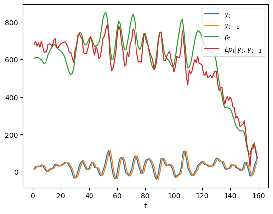
In the above graph, the green line is what the price of the stock would be if people had perfect foresight about the path of dividends while the red line is the conditional expectation \(E p_t | y_t, y_{t-1}\), which is what the price would be if people did not have perfect foresight but were optimally predicting future dividends on the basis of the information \(y_t, y_{t-1}\) at time \(t\).
13.12. Filtering foundations#
Assume that \(x_0\) is an \(n \times 1\) random vector and that \(y_0\) is a \(p \times 1\) random vector determined by the observation equation
where \(v_0\) is orthogonal to \(x_0\), \(G\) is a \(p \times n\) matrix, and \(R\) is a \(p \times p\) positive definite matrix.
We consider the problem of someone who
observes \(y_0\)
does not observe \(x_0\),
knows \(\hat x_0, \Sigma_0, G, R\) and therefore the joint probability distribution of the vector \(\begin{bmatrix} x_0 \cr y_0 \end{bmatrix}\)
wants to infer \(x_0\) from \(y_0\) in light of what he knows about that joint probability distribution.
Therefore, the person wants to construct the probability distribution of \(x_0\) conditional on the random vector \(y_0\).
The joint distribution of \(\begin{bmatrix} x_0 \cr y_0 \end{bmatrix}\) is multivariate normal \({\mathcal N}(\mu, \Sigma)\) with
By applying an appropriate instance of the above formulas for the mean vector \(\hat \mu_1\) and covariance matrix \(\hat \Sigma_{11}\) of \(z_1\) conditional on \(z_2\), we find that the probability distribution of \(x_0\) conditional on \(y_0\) is \({\mathcal N}(\tilde x_0, \tilde \Sigma_0)\) where
We can express our finding that the probability distribution of \(x_0\) conditional on \(y_0\) is \({\mathcal N}(\tilde x_0, \tilde \Sigma_0)\) by representing \(x_0\) as
where \(\zeta_0\) is a Gaussian random vector that is orthogonal to \(\tilde x_0\) and \(y_0\) and that has mean vector \(0\) and conditional covariance matrix \( E [\zeta_0 \zeta_0' | y_0] = \tilde \Sigma_0\).
13.12.1. Step toward dynamics#
Now suppose that we are in a time series setting and that we have the one-step state transition equation
where \(A\) is an \(n \times n\) matrix and \(C\) is an \(n \times m\) matrix.
Using equation (13.2), we can also represent \(x_1\) as
It follows that
and that the corresponding conditional covariance matrix \(E (x_1 - E x_1| y_0) (x_1 - E x_1| y_0)' \equiv \Sigma_1\) is
or
We can write the mean of \(x_1\) conditional on \(y_0\) as
or
where
13.12.2. Dynamic version#
Suppose now that for \(t \geq 0\), \(\{x_{t+1}, y_t\}_{t=0}^\infty\) are governed by the equations
where as before \(x_0 \sim {\mathcal N}(\hat x_0, \Sigma_0)\), \(w_{t+1}\) is the \(t+1\)th component of an i.i.d. stochastic process distributed as \(w_{t+1} \sim {\mathcal N}(0, I)\), and \(v_t\) is the \(t\)th component of an i.i.d. process distributed as \(v_t \sim {\mathcal N}(0, R)\) and the \(\{w_{t+1}\}_{t=0}^\infty\) and \(\{v_t\}_{t=0}^\infty\) processes are orthogonal at all pairs of dates.
The logic and formulas that we applied above imply that the probability distribution of \(x_t\) conditional on \(y_0, y_1, \ldots , y_{t-1} = y^{t-1}\) is
where \(\{\tilde x_t, \tilde \Sigma_t\}_{t=1}^\infty\) can be computed by iterating on the following equations starting from \(t=1\) and initial conditions for \(\tilde x_0, \tilde \Sigma_0\) computed as we have above:
If we shift the first equation forward one period and then substitute the expression for \(\tilde \Sigma_t\) on the right side of the fifth equation into it we obtain
This is a matrix Riccati difference equation that is closely related to another matrix Riccati difference equation that appears in a quantecon lecture on the basics of linear quadratic control theory.
That equation has the form
Stare at the two preceding equations for a moment or two, the first being a matrix difference equation for a conditional covariance matrix, the second being a matrix difference equation in the matrix appearing in a quadratic form for an intertemporal cost of value function.
Although the two equations are not identical, they display striking family resemblances.
the first equation tells dynamics that work forward in time
the second equation tells dynamics that work backward in time
while many of the terms are similar, one equation seems to apply matrix transformations to some matrices that play similar roles in the other equation
The family resemblences of these two equations reflects a transcendent duality that prevails between control theory and filtering theory.
13.12.3. An example#
We can use the Python class MultivariateNormal to construct examples.
Here is an example for a single period problem at time \(0\)
G = np.array([[1., 3.]])
R = np.array([[1.]])

x0_hat = np.array([0., 1.])
Σ0 = np.array([[1., .5], [.5, 2.]])

μ = np.hstack([x0_hat, G @ x0_hat])
Σ = np.block([[Σ0, Σ0 @ G.T], [G @ Σ0, G @ Σ0 @ G.T + R]])
# construction of the multivariate normal instance
multi_normal = MultivariateNormal(μ, Σ)
multi_normal.partition(2)
# the observation of y
y0 = 2.3

# conditional distribution of x0
μ1_hat, Σ11 = multi_normal.cond_dist(0, y0)
μ1_hat, Σ11
(array([-0.07608696,  0.80217391]),
 array([[ 0.72826087, -0.20652174],
        [-0.20652174,  0.16304348]]))
A = np.array([[0.5, 0.2], [-0.1, 0.3]])
C = np.array([[2.], [1.]])

# conditional distribution of x1
x1_cond = A @ μ1_hat
Σ1_cond = C @ C.T + A @ Σ11 @ A.T
x1_cond, Σ1_cond
(array([0.1223913 , 0.24826087]),
 array([[4.14728261, 1.94652174],
        [1.94652174, 1.03434783]]))
13.12.4. Code for iterating#
Here is code for solving a dynamic filtering problem by iterating on our equations, followed by an example.
def iterate(x0_hat, Σ0, A, C, G, R, y_seq):

    p, n = G.shape

    T = len(y_seq)
    x_hat_seq = np.empty((T+1, n))
    Σ_hat_seq = np.empty((T+1, n, n))

    x_hat_seq[0] = x0_hat
    Σ_hat_seq[0] = Σ0

    for t in range(T):
        xt_hat = x_hat_seq[t]
        Σt = Σ_hat_seq[t]
        μ = np.hstack([xt_hat, G @ xt_hat])
        Σ = np.block([[Σt, Σt @ G.T], [G @ Σt, G @ Σt @ G.T + R]])

        # filtering
        multi_normal = MultivariateNormal(μ, Σ)
        multi_normal.partition(n)
        x_tilde, Σ_tilde = multi_normal.cond_dist(0, y_seq[t])

        # forecasting
        x_hat_seq[t+1] = A @ x_tilde
        Σ_hat_seq[t+1] = C @ C.T + A @ Σ_tilde @ A.T

    return x_hat_seq, Σ_hat_seq
iterate(x0_hat, Σ0, A, C, G, R, [2.3, 1.2, 3.2])
(array([[0.        , 1.        ],
        [0.1223913 , 0.24826087],
        [0.18729801, 0.06881254],
        [0.75600369, 0.05547207]]),
 array([[[1.        , 0.5       ],
         [0.5       , 2.        ]],

        [[4.14728261, 1.94652174],
         [1.94652174, 1.03434783]],

        [[4.08853181, 1.98917687],
         [1.98917687, 1.00757802]],

        [[4.06650435, 1.99952946],
         [1.99952946, 1.00271293]]]))
The iterative algorithm just described is a version of the celebrated Kalman filter.
We describe the Kalman filter and some applications of it in A First Look at the Kalman Filter
13.13. Classic factor analysis model#
The factor analysis model can be represented as
where
\(Y\) is \(n \times 1\) random vector, \(E U U^\top = D\) is a diagonal matrix,
\(\Lambda\) is \(n \times k\) coefficient matrix,
\(f\) is \(k \times 1\) random vector, \(E f f^\top = I\),
\(U\) is \(n \times 1\) random vector, and \(U \perp f\) (i.e., \(E U f^\top = 0 \) )
It is presumed that \(k\) is small relative to \(n\); often \(k\) is only \(1\) or \(2\), as in our IQ examples.
This implies that
Thus, the covariance matrix \(\Sigma_Y\) is the sum of a diagonal matrix \(D\) and a positive semi-definite matrix \(\Lambda \Lambda^\top\) of rank \(k\).
This means that all covariances among the \(n\) components of the \(Y\) vector are intermediated by their common dependencies on the \(k\) factors.
Form
the covariance matrix of the expanded random vector \(Z\) can be computed as
In the following, we first construct the mean vector and the covariance matrix for the case where \(N=10\) and \(k=2\).
N = 10
k = 2
We set the coefficient matrix \(\Lambda\) and the covariance matrix of \(U\) to be
where the first half of the first column of \(\Lambda\) is filled with \(1\)s and \(0\)s for the rest half, and symmetrically for the second column.
\(D\) is a diagonal matrix with parameter \(\sigma_{u}^{2}\) on the diagonal.
Λ = np.zeros((N, k))
Λ[:N//2, 0] = 1
Λ[N//2:, 1] = 1

σu = .5
D = np.eye(N) * σu ** 2
# compute Σy
Σy = Λ @ Λ.T + D
We can now construct the mean vector and the covariance matrix for \(Z\).
μz = np.zeros(k+N)

Σz = np.empty((k+N, k+N))

Σz[:k, :k] = np.eye(k)
Σz[:k, k:] = Λ.T
Σz[k:, :k] = Λ
Σz[k:, k:] = Σy
z = rng.multivariate_normal(μz, Σz)

f = z[:k]
y = z[k:]
multi_normal_factor = MultivariateNormal(μz, Σz)
multi_normal_factor.partition(k)
Let’s compute the conditional distribution of the hidden factor \(f\) on the observations \(Y\), namely, \(f \mid Y=y\).
multi_normal_factor.cond_dist(0, y)
(array([0.14356426, 1.84615504]),
 array([[0.04761905, 0.        ],
        [0.        , 0.04761905]]))
We can verify that the conditional mean \(E \left[f \mid Y=y\right] = B Y\) where \(B = \Lambda^\top \Sigma_{y}^{-1}\).
B = Λ.T @ np.linalg.inv(Σy)

B @ y
array([0.14356426, 1.84615504])
Similarly, we can compute the conditional distribution \(Y \mid f\).
multi_normal_factor.cond_dist(1, f)
(array([0.41858317, 0.41858317, 0.41858317, 0.41858317, 0.41858317,
        2.04367341, 2.04367341, 2.04367341, 2.04367341, 2.04367341]),
 array([[0.25, 0.  , 0.  , 0.  , 0.  , 0.  , 0.  , 0.  , 0.  , 0.  ],
        [0.  , 0.25, 0.  , 0.  , 0.  , 0.  , 0.  , 0.  , 0.  , 0.  ],
        [0.  , 0.  , 0.25, 0.  , 0.  , 0.  , 0.  , 0.  , 0.  , 0.  ],
        [0.  , 0.  , 0.  , 0.25, 0.  , 0.  , 0.  , 0.  , 0.  , 0.  ],
        [0.  , 0.  , 0.  , 0.  , 0.25, 0.  , 0.  , 0.  , 0.  , 0.  ],
        [0.  , 0.  , 0.  , 0.  , 0.  , 0.25, 0.  , 0.  , 0.  , 0.  ],
        [0.  , 0.  , 0.  , 0.  , 0.  , 0.  , 0.25, 0.  , 0.  , 0.  ],
        [0.  , 0.  , 0.  , 0.  , 0.  , 0.  , 0.  , 0.25, 0.  , 0.  ],
        [0.  , 0.  , 0.  , 0.  , 0.  , 0.  , 0.  , 0.  , 0.25, 0.  ],
        [0.  , 0.  , 0.  , 0.  , 0.  , 0.  , 0.  , 0.  , 0.  , 0.25]]))
It can be verified that the mean is \(\Lambda I^{-1} f = \Lambda f\).
Λ @ f
array([0.41858317, 0.41858317, 0.41858317, 0.41858317, 0.41858317,
       2.04367341, 2.04367341, 2.04367341, 2.04367341, 2.04367341])
13.14. PCA and factor analysis#
To learn about Principal Components Analysis (PCA), please see this lecture Singular Value Decompositions.
For fun, let’s apply a PCA decomposition to a covariance matrix \(\Sigma_y\) that in fact is governed by our factor-analytic model.
Technically, this means that the PCA model is misspecified.
(Can you explain why?)
Nevertheless, this exercise will let us study how well the first two principal components from a PCA can approximate the conditional expectations \(E f_i | Y\) for our two factors \(f_i\), \(i=1,2\) for the factor analytic model that we have assumed truly governs the data on \(Y\) we have generated.
So we compute the PCA decomposition
where \(\tilde{\Lambda}\) is a diagonal matrix.
We have
and
Note that we will arrange the eigenvectors in \(P\) in the descending order of eigenvalues.
𝜆_tilde, P = np.linalg.eigh(Σy)

# arrange the eigenvectors by eigenvalues
ind = sorted(range(N), key=lambda x: 𝜆_tilde[x], reverse=True)

P = P[:, ind]
𝜆_tilde = 𝜆_tilde[ind]
Λ_tilde = np.diag(𝜆_tilde)

print('𝜆_tilde =', 𝜆_tilde)
𝜆_tilde = [5.25 5.25 0.25 0.25 0.25 0.25 0.25 0.25 0.25 0.25]
# verify the orthogonality of eigenvectors
np.abs(P @ P.T - np.eye(N)).max()
np.float64(4.440892098500626e-16)
# verify the eigenvalue decomposition is correct
P @ Λ_tilde @ P.T
array([[1.25, 1.  , 1.  , 1.  , 1.  , 0.  , 0.  , 0.  , 0.  , 0.  ],
       [1.  , 1.25, 1.  , 1.  , 1.  , 0.  , 0.  , 0.  , 0.  , 0.  ],
       [1.  , 1.  , 1.25, 1.  , 1.  , 0.  , 0.  , 0.  , 0.  , 0.  ],
       [1.  , 1.  , 1.  , 1.25, 1.  , 0.  , 0.  , 0.  , 0.  , 0.  ],
       [1.  , 1.  , 1.  , 1.  , 1.25, 0.  , 0.  , 0.  , 0.  , 0.  ],
       [0.  , 0.  , 0.  , 0.  , 0.  , 1.25, 1.  , 1.  , 1.  , 1.  ],
       [0.  , 0.  , 0.  , 0.  , 0.  , 1.  , 1.25, 1.  , 1.  , 1.  ],
       [0.  , 0.  , 0.  , 0.  , 0.  , 1.  , 1.  , 1.25, 1.  , 1.  ],
       [0.  , 0.  , 0.  , 0.  , 0.  , 1.  , 1.  , 1.  , 1.25, 1.  ],
       [0.  , 0.  , 0.  , 0.  , 0.  , 1.  , 1.  , 1.  , 1.  , 1.25]])
ε = P.T @ y

print("ε = ", ε)
ε =  [ 0.33707041  4.33453458  0.26386722 -0.39706296 -0.30020843  0.45473871
  0.19640695  0.07004059  0.35348891  0.81330557]
# print the values of the two factors

print('f = ', f)
f = [0.41858317 2.04367341]
Below we’ll plot several things
the \(N\) values of \(y\)
the \(N\) values of the principal components \(\epsilon\)
the value of the first factor \(f_1\) plotted only for the first \(N/2\) observations of \(y\) for which it receives a non-zero loading in \(\Lambda\)
the value of the second factor \(f_2\) plotted only for the final \(N/2\) observations for which it receives a non-zero loading in \(\Lambda\)
plt.scatter(range(N), y, label='y')
plt.scatter(range(N), ε, label=r'$\epsilon$')
plt.hlines(f[0], 0, N//2-1, ls='--', label='$f_{1}$')
plt.hlines(f[1], N//2, N-1, ls='-.', label='$f_{2}$')
plt.legend()

plt.show()
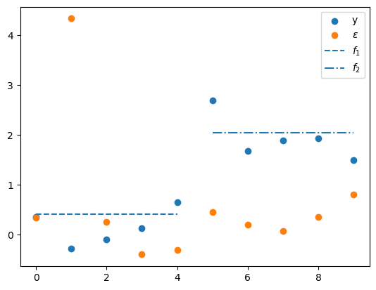
Consequently, the first two \(\epsilon_{j}\) correspond to the largest two eigenvalues.
Let’s look at them, after which we’ll look at \(E f | y = B y\)
ε[:2]
array([0.33707041, 4.33453458])
# compare with Ef|y
B @ y
array([0.14356426, 1.84615504])
Note
The two largest eigenvalues are both \(5.25\) in this example.
When an eigenvalue is repeated, the associated principal components are not individually pinned down: any orthonormal basis for the same two-dimensional eigenspace is valid.
For that reason, it is not meaningful to compare \(\epsilon_1\) and \(\epsilon_2\) component-by-component with \(E[f \mid Y]\).
The PC scores live in a PCA coordinate system, while \(E[f \mid Y]\) lives in factor space.
Even within the common two-dimensional subspace, the PCA basis can be rotated or sign-flipped, and its coordinates need not use the same scaling as the factor coordinates.
What is uniquely determined is the two-dimensional subspace spanned by the first two columns of \(P\).
In this symmetric example, that subspace is exactly the column space of \(\Lambda\).
The fraction of variance in \(y_t\) explained by the first two principal components is
𝜆_tilde[:2].sum() / 𝜆_tilde.sum()
np.float64(0.84)
To compare PCA with the factor model in observation space, compute
where \(P_j\) and \(P_k\) are the eigenvectors associated with the two largest eigenvalues.
y_hat = P[:, :2] @ ε[:2]
\(\hat{Y}\) is the rank-2 PCA approximation to \(Y\) in observation space, so it is a 10-vector rather than a 2-vector.
The natural observation-space counterpart from the factor model is \(\Lambda E[f \mid Y]\), which is also a 10-vector.
In this symmetric example, both vectors lie in the same two-dimensional subspace, namely the column space of \(\Lambda\).
They are therefore close, but not identical.
The PCA reconstruction uses the block means directly, while \(\Lambda E[f \mid Y]\) shrinks those block means toward zero by the factor \(5/(5+\sigma_u^2) \approx 0.952\).
The next plot makes this comparison concrete.
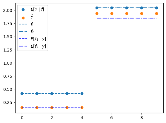
The two scatter plots, \(E[Y \mid f] = \Lambda f\) and \(\hat{Y}\), are both 10-vectors in observation space, so they can be compared directly.
The horizontal lines show the factor values \(f_1\) and \(f_2\), together with their posterior means \(E[f_i \mid Y]\).
These are 2-dimensional factor-space quantities, drawn over the relevant half of the index set to match the block structure of \(\Lambda\).
This uses the same idea as the earlier formula \(E[Y \mid f] = \Lambda f\): the matrix \(\Lambda\) maps a 2-vector in factor space into a 10-vector in observation space.
In our example,
because the first five rows of \(\Lambda\) are \((1,0)\) and the last five rows are \((0,1)\).
Therefore, once we observe \(Y=y\), the posterior mean \(E[f \mid Y=y] = \begin{bmatrix} E[f_1 \mid y] \\ E[f_2 \mid y] \end{bmatrix}\) is converted into the observation-space vector
So the horizontal line at height \(E[f_1 \mid y]\) over the first five indices, together with the horizontal line at height \(E[f_2 \mid y]\) over the last five indices, is exactly a picture of \(\Lambda E[f \mid Y=y]\).
plt.scatter(range(N), Λ @ f, label=r'$E[Y \mid f]$')
plt.scatter(range(N), y_hat, label=r'$\hat{Y}$')
plt.hlines(f[0], 0, N//2-1, ls='--', label='$f_{1}$')
plt.hlines(f[1], N//2, N-1, ls='-.', label='$f_{2}$')

Efy = B @ y
plt.hlines(Efy[0], 0, N//2-1, ls='--', color='b', label=r'$E[f_1 \mid y]$')
plt.hlines(Efy[1], N//2, N-1, ls='-.', color='b', label=r'$E[f_2 \mid y]$')
plt.legend()

plt.show()
To compute the covariance matrix of \(\hat{Y}\), first form the covariance matrix of \(\epsilon\) and then extract the upper-left block corresponding to \(\epsilon_1\) and \(\epsilon_2\).
Σεjk = (P.T @ Σy @ P)[:2, :2]

Pjk = P[:, :2]

Σy_hat = Pjk @ Σεjk @ Pjk.T
print('Σy_hat = \n', Σy_hat)
Σy_hat =
 [[1.05 1.05 1.05 1.05 1.05 0.   0.   0.   0.   0.  ]
 [1.05 1.05 1.05 1.05 1.05 0.   0.   0.   0.   0.  ]
 [1.05 1.05 1.05 1.05 1.05 0.   0.   0.   0.   0.  ]
 [1.05 1.05 1.05 1.05 1.05 0.   0.   0.   0.   0.  ]
 [1.05 1.05 1.05 1.05 1.05 0.   0.   0.   0.   0.  ]
 [0.   0.   0.   0.   0.   1.05 1.05 1.05 1.05 1.05]
 [0.   0.   0.   0.   0.   1.05 1.05 1.05 1.05 1.05]
 [0.   0.   0.   0.   0.   1.05 1.05 1.05 1.05 1.05]
 [0.   0.   0.   0.   0.   1.05 1.05 1.05 1.05 1.05]
 [0.   0.   0.   0.   0.   1.05 1.05 1.05 1.05 1.05]]
13.15. Exercises#
Exercise 13.1
Verify conditional mean and variance by simulation
For the bivariate normal with
fix \(z_2 = 2\).
Use
MultivariateNormalto compute the analytical conditional mean \(\hat{\mu}_1\) and variance \(\hat{\Sigma}_{11}\) of \(z_1 \mid z_2 = 2\).Draw \(10^6\) samples from the joint distribution.
Retain only those for which \(|z_2 - 2| < 0.05\).
Compute the sample mean and variance of the retained \(z_1\) values.
Confirm that the sample estimates are close to the analytical values.
Solution
Here is one solution:
μ = np.array([.5, 1.])
Σ = np.array([[1., .5], [.5, 1.]])

mn = MultivariateNormal(μ, Σ)
mn.partition(1)
μ1_hat, Σ11_hat = mn.cond_dist(0, np.array([2.]))
print(f"Analytical  μ1_hat = {μ1_hat[0]:.4f},  Σ11_hat = {Σ11_hat[0,0]:.4f}")

n = 1_000_000
data = rng.multivariate_normal(μ, Σ, size=n)
z1_all, z2_all = data[:, 0], data[:, 1]

mask = np.abs(z2_all - 2.) < 0.05
z1_cond = z1_all[mask]
print(f"Sample size in band: {mask.sum()}")
print(f"Sample      μ1_hat = {np.mean(z1_cond):.4f},  Σ11_hat = {np.var(z1_cond, ddof=1):.4f}")
Analytical  μ1_hat = 1.0000,  Σ11_hat = 0.7500
Sample size in band: 24314
Sample      μ1_hat = 1.0050,  Σ11_hat = 0.7458
Exercise 13.2
Product of regression slopes equals squared correlation
For a bivariate normal with standard deviations \(\sigma_1 = \sigma_2 = 1\) and correlation \(\rho\), show analytically that \(b_1 b_2 = \rho^2\), where \(b_1\) is the slope of \(z_1\) on \(z_2\) and \(b_2\) is the slope of \(z_2\) on \(z_1\).
Then verify numerically for \(\rho \in \{0.2, 0.5, 0.9\}\) that
βs[0] * βs[1] \(= \rho^2\) by constructing the appropriate
MultivariateNormal instances.
Solution
The regression slopes are
so \(b_1 b_2 = \rho^2\).
for ρ in [0.2, 0.5, 0.9]:
    Σ = np.array([[1., ρ], [ρ, 1.]])
    mn = MultivariateNormal(np.zeros(2), Σ)
    mn.partition(1)
    product = mn.βs[0].item() * mn.βs[1].item()
    print(f"ρ={ρ:.1f}:  b1*b2 = {product:.4f}")
    print(f"ρ^2 = {ρ**2:.4f},  match: {np.isclose(product, ρ**2)}")
ρ=0.2:  b1*b2 = 0.0400
ρ^2 = 0.0400,  match: True
ρ=0.5:  b1*b2 = 0.2500
ρ^2 = 0.2500,  match: True
ρ=0.9:  b1*b2 = 0.8100
ρ^2 = 0.8100,  match: True
Exercise 13.3
IQ inference: effect of the signal-to-noise ratio
Using the one-dimensional IQ model with \(n = 50\) test scores and \(\mu_\theta = 100\), \(\sigma_\theta = 10\):
Vary the test-score noise \(\sigma_y \in \{1, 5, 10, 20, 50\}\).
For each value, plot the posterior standard deviation \(\hat{\sigma}_\theta\) as a function of the number of test scores included (from 1 to 50), with all curves on the same axes.
Explain intuitively why a larger \(\sigma_y\) leads to a slower decline of posterior uncertainty.
Solution
Here is one solution:
n_max = 50
μθ_val, σθ_val = 100., 10.

fig, ax = plt.subplots()
for σy_val in [1., 5., 10., 20., 50.]:
    σθ_hat_arr = np.empty(n_max)
    for i in range(1, n_max + 1):
        μ_i, Σ_i, _ = construct_moments_IQ(i, μθ_val, σθ_val, σy_val)
        mn_i = MultivariateNormal(μ_i, Σ_i)
        mn_i.partition(i)
        _, Σθ_i = mn_i.cond_dist(1, np.zeros(i))
        σθ_hat_arr[i - 1] = np.sqrt(Σθ_i[0, 0])
    ax.plot(range(1, n_max + 1), σθ_hat_arr, label=f'σy={σy_val:.0f}')

ax.set_xlabel('number of test scores')
ax.set_ylabel(r'posterior $\hat{\sigma}_\theta$')
ax.legend()
plt.show()
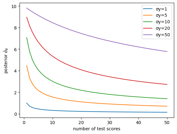
When \(\sigma_y\) is large each test score is a noisy signal about \(\theta\), so many more observations are required before the posterior variance falls appreciably.
In the limit \(\sigma_y \to 0\) a single observation pins down \(\theta\) exactly.
Exercise 13.4
Prior vs. likelihood in IQ inference
Using the one-dimensional IQ model with \(n = 20\) test scores and \(\mu_\theta = 100\), \(\sigma_y = 10\):
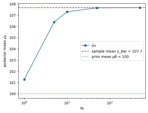
Fix \(\sigma_y = 10\) and vary the prior spread \(\sigma_\theta \in \{1, 5, 10, 50, 500\}\).
For each value compute the posterior mean \(\hat{\mu}_\theta\) given the same set of \(n = 20\) test scores and plot \(\hat{\mu}_\theta\) against \(\sigma_\theta\).
Show analytically (or verify numerically) that
as \(\sigma_\theta \to \infty\) the posterior mean converges to the sample mean \(\bar{y}\) (the data dominate the prior), and
as \(\sigma_\theta \to 0\) the posterior mean converges to the prior mean \(\mu_\theta\) (the prior dominates the data).
Hint
The posterior mean formula is \(\hat{\mu}_\theta = \bigl(\mu_\theta/\sigma_\theta^2 + n\bar{y}/\sigma_y^2\bigr) \big/ \bigl(1/\sigma_\theta^2 + n/\sigma_y^2\bigr)\).
Examine each limit by letting \(\sigma_\theta\) go to \(\infty\) or \(0\).
Solution
Here is one solution:
n_scores = 20
μθ_val, σy_val = 100., 10.

rng = np.random.default_rng(42)
true_θ = 108.
y_obs = true_θ + σy_val * rng.standard_normal(n_scores)
y_bar = np.mean(y_obs)

σθ_vals = [1., 5., 10., 50., 500.]
μθ_hat_vals = []

for σθ_val in σθ_vals:
    μ_i, Σ_i, _ = construct_moments_IQ(n_scores, μθ_val, σθ_val, σy_val)
    mn_i = MultivariateNormal(μ_i, Σ_i)
    mn_i.partition(n_scores)
    μθ_hat, _ = mn_i.cond_dist(1, y_obs)
    μθ_hat_vals.append(μθ_hat.item())

def posterior_mean(σθ_val):
    μ_i, Σ_i, _ = construct_moments_IQ(n_scores, μθ_val, σθ_val, σy_val)
    mn_i = MultivariateNormal(μ_i, Σ_i)
    mn_i.partition(n_scores)
    μθ_hat, _ = mn_i.cond_dist(1, y_obs)
    return μθ_hat.item()

fig, ax = plt.subplots()
ax.semilogx(σθ_vals, μθ_hat_vals, 'o-',
            label=r'$\hat{\mu}_\theta$')
ax.axhline(y_bar,  ls='--', color='r',
            label=f'sample mean y_bar = {y_bar:.1f}')
ax.axhline(μθ_val, ls=':',  color='g',
            label=f'prior mean μθ = {μθ_val:.0f}')
ax.set_xlabel(r'$\sigma_\theta$')
ax.set_ylabel(r'posterior mean $\hat{\mu}_\theta$')
ax.legend()
plt.show()

σθ_small = 1e-2
σθ_large = 1e4

print(f"y_bar = {y_bar:.4f}")
print(f"Posterior mean with σθ={σθ_large:.0e}: {posterior_mean(σθ_large):.4f}")
print(f"Posterior mean with σθ={σθ_small:.0e}: {posterior_mean(σθ_small):.4f}")
print(f"Prior mean μθ = {μθ_val:.4f}")
y_bar = 107.6707
Posterior mean with σθ=1e+04: 107.6707
Posterior mean with σθ=1e-02: 100.0002
Prior mean μθ = 100.0000
Exercise 13.5
Kalman filter convergence
Using the iterate function from the Filtering Foundations section with
and initial conditions \(\hat{x}_0 = [0, 0]'\), \(\Sigma_0 = I_2\):
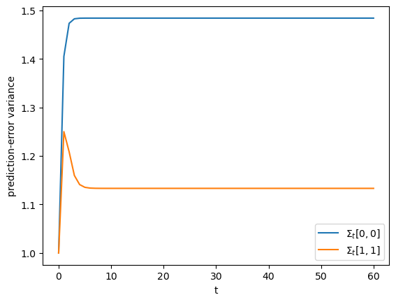
Simulate \(T = 60\) periods of \(\{x_t, y_t\}\) and run the filter.
Plot the sequences of conditional variances \(\Sigma_t[0,0]\) and \(\Sigma_t[1,1]\) over time.
Verify that they converge to a steady state.
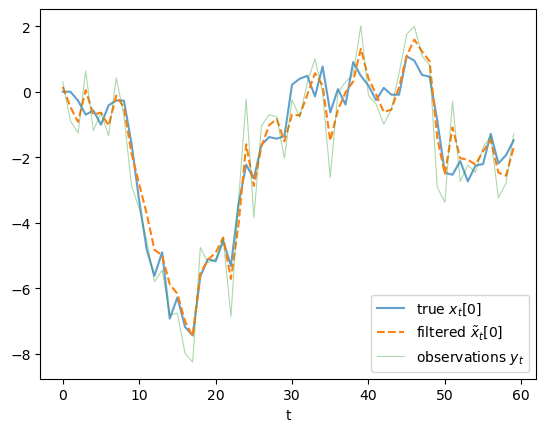
Plot the filtered state estimates \(\tilde{x}_t[0]\) together with the true \(x_t[0]\) and the raw observations \(y_t\) on a single figure.
Solution
Here is one solution:
A_ex = np.array([[0.9, 0.], [0., 0.5]])
C_ex = np.array([[1.], [1.]])
G_ex = np.array([[1., 0.]])
R_ex = np.array([[1.]])

T_ex = 60
x0_hat_ex = np.zeros(2)
Σ0_ex = np.eye(2)

rng = np.random.default_rng(7)
x_true = np.zeros((T_ex + 1, 2))
y_seq_ex = np.zeros(T_ex)
for t in range(T_ex):
    x_true[t + 1] = A_ex @ x_true[t] + C_ex[:, 0] * rng.standard_normal()
    y_seq_ex[t] = (G_ex @ x_true[t]).item() + rng.standard_normal()

x_hat_seq, Σ_hat_seq = iterate(
    x0_hat_ex, Σ0_ex, A_ex, C_ex, G_ex, R_ex, y_seq_ex)

# x_hat_seq[t] = E[x_t | y^{t-1}] (one-step-ahead prediction)
# Σ_hat_seq[t] = corresponding prediction-error covariance
fig, ax = plt.subplots()
ax.plot(Σ_hat_seq[:, 0, 0], label=r'$\Sigma_t[0,0]$')
ax.plot(Σ_hat_seq[:, 1, 1], label=r'$\Sigma_t[1,1]$')
ax.set_xlabel('t')
ax.set_ylabel('prediction-error variance')
ax.legend()
plt.show()

# The `iterate` function stores one-step-ahead predictions.
# We recover the filtered estimates E[x_t | y^t] by re-applying
# the measurement-update step at each t.
n_state = 2
x_filt_seq = np.empty((T_ex, n_state))
for t in range(T_ex):
    xt_hat = x_hat_seq[t]
    Σt     = Σ_hat_seq[t]
    μ_k = np.hstack([xt_hat, G_ex @ xt_hat])
    Σ_k = np.block([[Σt,          Σt  @ G_ex.T          ],
                    [G_ex @ Σt,   G_ex @ Σt @ G_ex.T + R_ex]])
    mn_k = MultivariateNormal(μ_k, Σ_k)
    mn_k.partition(n_state)
    x_filt_seq[t], _ = mn_k.cond_dist(0, y_seq_ex[t:t+1])

fig, ax = plt.subplots()
ax.plot(x_true[:-1, 0], label='true $x_t[0]$', alpha=0.7)
ax.plot(x_filt_seq[:, 0], label=r'filtered $\tilde{x}_t[0]$', ls='--')
ax.plot(y_seq_ex, label='observations $y_t$', alpha=0.4, lw=0.8)
ax.set_xlabel('t')
ax.legend()
plt.show()
Exercise 13.6
PCA vs. factor analysis
In the classic factor analysis model at the end of the lecture the true covariance is \(\Sigma_y = \Lambda \Lambda' + D\).
Set \(\sigma_u = 2\) (instead of \(0.5\)).
Recompute the fraction of variance explained by the first two principal components and compare it with the \(\sigma_u = 0.5\) result.
Explain the change.
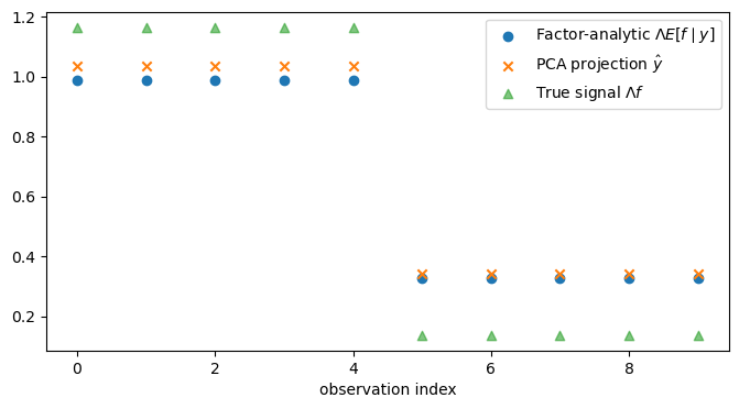
Show that the observation-space factor-analytic posterior \(\Lambda E[f \mid Y] = \Lambda B Y\) (an \(N\)-vector) is not equal to the two-component PCA reconstruction \(\hat{Y} = P_{:,1:2}\,\epsilon_{1:2}\) (also an \(N\)-vector).
Plot both on the same axes.
Note: \(E[f \mid Y] = BY\) is a \(k\)-vector and \(\hat{Y}\) is an \(N\)-vector, so they cannot be compared directly; the comparison must be made in observation space via \(\Lambda E[f \mid Y]\).
In one or two sentences, explain why PCA is misspecified for factor-analytic data.
Solution
Here is one solution:
rng = np.random.default_rng(42)

N_fa = 10
k_fa = 2

Λ_fa = np.zeros((N_fa, k_fa))
Λ_fa[:N_fa//2, 0] = 1
Λ_fa[N_fa//2:, 1] = 1

for σu_val in [0.5, 2.0]:
    D_fa = np.eye(N_fa) * σu_val ** 2
    Σy_fa = Λ_fa @ Λ_fa.T + D_fa

    λ_fa, P_fa = np.linalg.eigh(Σy_fa)
    ind_fa = sorted(range(N_fa), key=lambda x: λ_fa[x], reverse=True)
    P_fa   = P_fa[:, ind_fa]
    λ_fa   = λ_fa[ind_fa]

    frac = λ_fa[:2].sum() / λ_fa.sum()
    print(f"σu={σu_val}: fraction explained by first 2 PCs = {frac:.4f}")

σu_b = 0.5
D_b = np.eye(N_fa) * σu_b ** 2
Σy_b = Λ_fa @ Λ_fa.T + D_b

μz_b = np.zeros(k_fa + N_fa)
Σz_b = np.block([[np.eye(k_fa), Λ_fa.T], [Λ_fa, Σy_b]])
z_b = rng.multivariate_normal(μz_b, Σz_b)
f_b = z_b[:k_fa]
y_b = z_b[k_fa:]

B_b = Λ_fa.T @ np.linalg.inv(Σy_b)
Efy_b  = B_b @ y_b

λ_b, P_b = np.linalg.eigh(Σy_b)
ind_b = sorted(range(N_fa), key=lambda x: λ_b[x], reverse=True)
P_b = P_b[:, ind_b]
ε_b = P_b.T @ y_b
y_hat_b = P_b[:, :2] @ ε_b[:2]

fig, ax = plt.subplots(figsize=(8, 4))
ax.scatter(range(N_fa),
        Λ_fa @ Efy_b, label=r'Factor-analytic $\Lambda E[f\mid y]$')
ax.scatter(range(N_fa),
        y_hat_b, marker='x', label=r'PCA projection $\hat{y}$')
ax.scatter(range(N_fa),
        Λ_fa @ f_b, marker='^', alpha=0.6, label=r'True signal $\Lambda f$')
ax.set_xlabel('observation index')
ax.legend()
plt.show()
σu=0.5: fraction explained by first 2 PCs = 0.8400
σu=2.0: fraction explained by first 2 PCs = 0.3600
In this symmetric example, PCA does recover the same two-dimensional observation-space subspace as the factor model, namely the column space of \(\Lambda\). But PCA is still misspecified for factor-analytic data, because it treats the covariance matrix as an arbitrary matrix to be approximated and does not use the special decomposition \(\Sigma_y = \Lambda \Lambda^\top + D\) into a common part and an idiosyncratic noise part.
So the two methods are solving different problems. PCA forms \(\hat{Y}\) as the best rank-2 approximation to the observed data vector \(Y\), which in this example amounts to using the block means. The factor model instead computes \(\Lambda E[f \mid Y]\), the conditional mean of the latent common component \(\Lambda f\) given the data, and because it accounts for noise it shrinks those block means toward zero.