105. Priors, Escapes, and Learning Cycles#
105.1. Overview#
The Bourbons remember everything and learn nothing.
– Charles Maurice de Talleyrand
This lecture is a sequel to Adaptive Learning and Escape Dynamics.
It follows [Sargent and Williams, 2005], which generalizes the adaptive model of chapter 8 of [Sargent, 1999] and of [Cho et al., 2002] (CWS), whose escape dynamics we derived in Escaping Nash Inflation.
In Adaptive Learning and Escape Dynamics the government estimated its Phillips curve by recursive least squares.
That is a very particular way to learn.
A least squares learner behaves as if it believes that the coefficients of its model follow a specific random walk — one with a specific innovation covariance matrix.
Here we free the government to hold any prior about how its coefficients drift, encoded in a covariance matrix \(V\), and we ask how the shape of that prior affects the two forces that drive the model:
the mean dynamics, which pull the government’s beliefs toward a self-confirming (Nash) equilibrium; and
the escape dynamics, which occasionally push beliefs away from it, toward the low-inflation Ramsey outcome.
We will find three things.
Some priors make the self-confirming equilibrium unstable, so that the mean dynamics themselves produce recurrent disinflations — a learning cycle born of a Hopf bifurcation, rather than a rare stochastic escape.
The prior shapes the direction and speed of escapes; but in every case the escape heads toward the Ramsey outcome.
The prior explains a long-standing puzzle: why the simulations of Sims and Chung escape Nash inflation and stay near Ramsey forever, while those of [Sargent, 1999] and CWS escape only to be pulled back.
Throughout we work with the analytically tractable static model of Escaping Nash Inflation, in which the government runs a simple regression of unemployment on inflation and a constant.
Let’s start with our imports:
import matplotlib.pyplot as plt
import numpy as np
from scipy.linalg import sqrtm
from scipy.integrate import solve_ivp
105.2. The static model#
The true economy is a version of the natural-rate model of [Kydland and Prescott, 1977]:
where \(U_n\) is unemployment, \(\pi_n\) is inflation, \(x_n\) is the systematic part of inflation set by the government, \(\hat x_n\) is the public’s (rational) forecast, and \(W_n = (W_{1n}, W_{2n})^\top\) is IID standard Gaussian noise.
Since \(\pi_n - \hat x_n = \sigma_2 W_{2n}\), the true unemployment rate is \(U_n = u - \sigma_2 W_{2n} + \sigma_1 W_{1n}\) — it fluctuates around the natural rate \(u\) regardless of systematic policy.
The government does not know this.
In the static model it fits a non-expectational Phillips curve by regressing unemployment on current inflation and a constant,
with belief vector \(\gamma = (a, b)\) (intercept and slope), and it treats \(\eta_n\) as an exogenous shock.
Warning
Escaping Nash Inflation studies this same static model but orders the belief vector the other way round, as \(\gamma = (\gamma_1, \gamma_{-1})\) with the slope first and regressors \(\Phi = (\pi, 1)\), following [Cho et al., 2002].
Here we put the intercept first, with \(\Phi = (1, \pi)\), following [Sargent and Williams, 2005].
The two are the same model in different coordinates: \(a = \gamma_{-1}\) and \(b = \gamma_1\), so the self-confirming belief \((2u, -1)\) of this lecture is the \((-1, u(1+\theta^2))\) of the last one, with \(\theta = 1\).
Matrices such as \(M\), \(V\), and \(P\) have their rows and columns correspondingly transposed.
Believing (105.2), the government solves the Phelps problem — minimize \(\hat{\mathbb{E}} \sum_n \delta^n (U_n^2 + \pi_n^2)\) — whose static best response sets inflation to the constant
class StaticPhillips:
    "The static Sargent-Williams model: government regresses U on (1, π)."

    def __init__(self, u=5.0, σ1=0.3, σ2=0.3):
        self.u, self.σ1, self.σ2 = u, σ1, σ2
        self.σ = σ1                       # govt regression error std = σ1

    def x(self, γ):
        "Government best response (systematic inflation) given beliefs γ."
        a, b = γ
        return -a * b / (1 + b**2)

    def M(self, γ):
        "Second moment matrix E[ΦΦ'] of regressors Φ = (1, π), given γ."
        x = self.x(γ)
        return np.array([[1.0, x], [x, x**2 + self.σ2**2]])

    def g_bar(self, γ):
        "Least squares moment E[Φ(U - Φ'γ)] under the data γ generates."
        u, σ2 = self.u, self.σ2
        x = self.x(γ)
        E_ΦU = np.array([u, x * u - σ2**2])
        return E_ΦU - self.M(γ) @ γ
Three belief vectors are worth naming.
Belief 1 (Nash): \(b = -1\) with an intercept that makes the government set \(x = u\), the time-consistent outcome of [Kydland and Prescott, 1977].
Belief 2 (Ramsey): \(b = 0\), so the government perceives no tradeoff and sets \(x = 0\).
Belief 3 (induction): in a dynamic version, coefficients on current and lagged inflation summing to zero, which for a patient government also sends inflation toward \(0\).
105.3. The self-confirming equilibrium#
A self-confirming equilibrium is a belief \(\bar\gamma\) that reproduces itself: the data generated when the government acts on \(\bar\gamma\) make the population regression coefficients equal \(\bar\gamma\), i.e. \(\bar g(\bar\gamma) = 0\).
For the static model this is easy to solve by hand.
The slope is \(b = \operatorname{cov}(U, \pi)/\mathbb{V}[\pi] = -\sigma_2^2/\sigma_2^2 = -1\), and matching means gives the intercept \(a = u + x(\bar\gamma)\).
Substituting the best response (105.3) with \(b = -1\) gives \(x = a/2\), so \(a = u + a/2\), i.e. \(a = 2u\).
model = StaticPhillips(u=5.0, σ1=0.3, σ2=0.3)
γ_sce = np.array([2 * model.u, -1.0])

print(f"self-confirming beliefs  γ = {γ_sce}  (intercept 2u, slope -1)")
print(f"self-confirming inflation x = {model.x(γ_sce):.2f}  (= Nash = u)")
print(f"check g_bar(γ_sce) = {model.g_bar(γ_sce)}")
self-confirming beliefs  γ = [10. -1.]  (intercept 2u, slope -1)
self-confirming inflation x = 5.00  (= Nash = u)
check g_bar(γ_sce) = [0. 0.]
The self-confirming equilibrium inflation rate equals the Nash (time-consistent) outcome \(u = 5\), even though the government’s model is misspecified.
The government’s non-expectational Phillips curve is observationally equivalent to the truth along the equilibrium path, but wrong off it — which is exactly what its adaptive behavior repeatedly probes.
105.4. Drifting beliefs and the Kalman filter#
We now make the government adaptive.
Following [Sargent and Williams, 2005], the government believes that the coefficients of its Phillips curve drift as a random walk,
and it forms its estimate \(\gamma_n = \hat\alpha_{n \mid n-1}\) by the Kalman filter.
The covariance matrix \(V\) is the government’s prior about parameter drift — the object we set free.
With regressors \(\Phi_n = (1, \pi_n)^\top\), a large-sample approximation to the Kalman filter (see [Benveniste et al., 1990]) is
where \(\sigma^2\) is the variance the government attributes to its regression error \(\eta_n\).
For a fixed \(\gamma\), the matrix \(P_n\) settles at the solution of the algebraic Riccati equation
The connection to Adaptive Learning and Escape Dynamics is exact.
Constant-gain recursive least squares is the special case in which the government’s prior is \(V = V^* \equiv \epsilon^2 \sigma^2 M(\bar\gamma)^{-1}\) and \(\sigma = \sigma_1\); then (105.6) gives \(P = \epsilon M(\bar\gamma)^{-1}\), and (105.5) reduces to the recursive least squares algorithm of the previous lecture, with gain \(\epsilon\).
def solve_riccati(V, M, σ):
    "Symmetric positive-definite P solving P M P = σ^{-2} V."
    W = V / σ**2
    Mh = sqrtm(M).real
    Mh_inv = np.linalg.inv(Mh)
    return Mh_inv @ sqrtm(Mh @ W @ Mh).real @ Mh_inv

M_sce = model.M(γ_sce)
V_star = model.σ**2 * np.linalg.inv(M_sce)      # the RLS prior (ε = 1)
P_star = solve_riccati(V_star, M_sce, model.σ)

print("RLS prior gives P = M^{-1}?", np.allclose(P_star, np.linalg.inv(M_sce)))
RLS prior gives P = M^{-1}? True
105.5. Mean dynamics and E-stability#
As in Adaptive Learning and Escape Dynamics, the beliefs are organized by mean dynamics — now a joint ordinary differential equation in \((\gamma, P)\),
A rest point of (105.7) has \(\bar g(\gamma) = 0\) and \(P = \) the Riccati solution — a self-confirming equilibrium.
Local stability turns on the Jacobian of \(\bar g\) at the self-confirming equilibrium.
For the static model this can be computed in closed form,
def jacobian(model, γ, h=1e-6):
    "Numerical Jacobian of g_bar at γ."
    J = np.zeros((2, 2))
    for j in range(2):
        gp, gm = γ.copy(), γ.copy()
        gp[j] += h; gm[j] -= h
        J[:, j] = (model.g_bar(gp) - model.g_bar(gm)) / (2 * h)
    return J

J = jacobian(model, γ_sce)
print("∂g/∂γ at SCE =\n", J.round(3))
∂g/∂γ at SCE =
 [[ -0.5   -5.  ]
 [ -2.5  -25.09]]
Under recursive least squares the \(P\) block of (105.7) decouples, and stability is governed by the eigenvalues of \(M^{-1}\,\partial\bar g/\partial\gamma\) — the classic E-stability condition of [Evans and Honkapohja, 2001].
eig_rls = np.linalg.eigvals(np.linalg.inv(M_sce) @ J)
print(f"E-stability eigenvalues (RLS): {eig_rls.round(3)}")
print("both negative ⇒ the SCE is E-stable, and least squares converges to Nash")
E-stability eigenvalues (RLS): [-0.5 -1. ]
both negative ⇒ the SCE is E-stable, and least squares converges to Nash
Both eigenvalues are negative — one of them exactly \(-\tfrac12\), the marginal value that appeared in Adaptive Learning and Escape Dynamics.
Under least squares, then, beliefs converge to the Nash self-confirming equilibrium.
But this reduction relied on the special RLS prior.
Under a general prior \(V\), the \(P\) block does not decouple, and stability is instead governed by the eigenvalues of \(\bar P\, \partial\bar g/\partial\gamma\) — where \(\bar P\) is the Riccati solution for that prior.
Prior beliefs about parameter drift now matter for whether the self-confirming equilibrium is even stable.
105.6. Learning cycles#
Here is the paper’s most striking result: some priors make the self-confirming equilibrium unstable, and a stable limit cycle is born through a Hopf bifurcation.
We illustrate it by tightening the government’s prior on the slope coefficient, starting from the RLS prior \(V^*\) and shrinking the slope-related entries by a factor \(\lambda \in [0, 1]\):
For each \(\lambda\) we solve the Riccati equation and look at the largest real part among the eigenvalues of \(\bar P(\lambda)\, \partial\bar g/\partial\gamma\): where it is positive, the self-confirming equilibrium is unstable.
def V_tighten_slope(λ, V_star):
    V = V_star.copy()
    V[0, 1] = V[1, 0] = np.sqrt(λ) * V_star[0, 1]
    V[1, 1] = λ * V_star[1, 1]
    return V

ε = 0.05                                   # gain (sets the timescale)
λ_grid = np.linspace(0.01, 0.999, 200)
max_re = []
for λ in λ_grid:
    V = ε**2 * V_tighten_slope(λ, V_star)
    P = solve_riccati(V, M_sce, model.σ)
    max_re.append(np.linalg.eigvals(P @ J).real.max())

fig, ax = plt.subplots(figsize=(8, 4.5))
ax.plot(λ_grid, max_re)
ax.axhline(0, color='k', lw=0.8)
ax.set_xlabel(r'prior-tightening parameter $\lambda$')
ax.set_ylabel('max real part of eigenvalue')
plt.show()
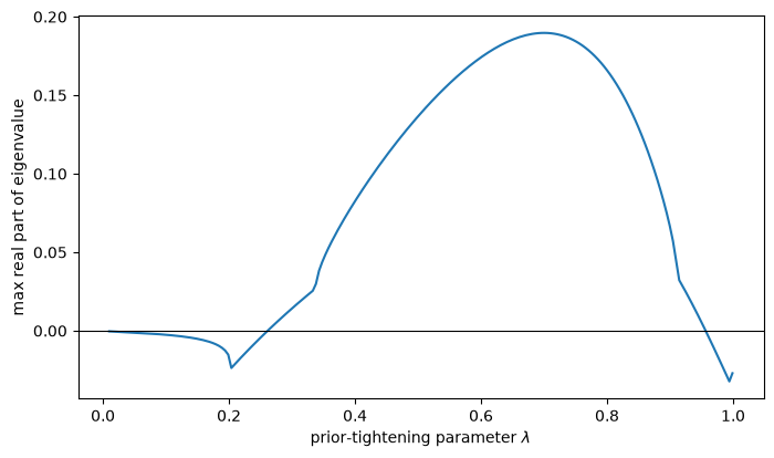
Fig. 105.1 Stability of the self-confirming equilibrium as the slope prior tightens#
Over an intermediate range of \(\lambda\) the maximum real part becomes positive: the self-confirming equilibrium loses stability.
By the Hopf bifurcation theorem (see [Perko, 1996]), a unique stable limit cycle bifurcates as the real parts cross zero — what [Bullard, 1994] calls a learning equilibrium.
Let’s integrate the mean dynamics for the regression coefficients at \(\lambda = 0.7\) (well inside the unstable range), holding \(P\) at its Riccati value, and trace the cycle.
λ = 0.7
V = ε**2 * V_tighten_slope(λ, V_star)
P_bar = solve_riccati(V, M_sce, model.σ)

def coeff_ode(t, γ):
    return P_bar @ model.g_bar(γ)

sol = solve_ivp(coeff_ode, [0, 2500], γ_sce + np.array([0.3, 0.05]),
                max_step=1.0, rtol=1e-9, atol=1e-11, dense_output=True)
a_path, b_path = sol.y
x_path = -a_path * b_path / (1 + b_path**2)

# isolate one mature cycle for the phase plot
mask = sol.t > sol.t[-1] - 800
fig, axes = plt.subplots(1, 2, figsize=(12, 5))

axes[0].plot(sol.t[mask], a_path[mask], label='intercept', lw=2)
axes[0].plot(sol.t[mask], b_path[mask], label='slope', lw=2)
axes[0].set_xlabel('time')
axes[0].set_ylabel('coefficient')
axes[0].set_title('Figure 5a: coefficients cycle')
axes[0].legend()

axes[1].plot(a_path[mask], b_path[mask], lw=2)
axes[1].plot(*γ_sce, 'kx', ms=10, label='SCE')
axes[1].set_xlabel('intercept')
axes[1].set_ylabel('slope')
axes[1].set_title('Figure 5b: the limit cycle')
axes[1].legend()

plt.tight_layout()
plt.show()
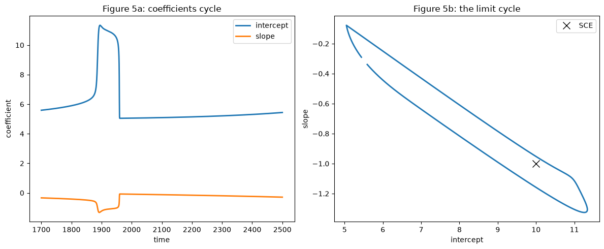
Fig. 105.2 Coefficients cycle, and the limit cycle in belief space#
The beliefs settle into a closed orbit around the self-confirming equilibrium.
Because inflation is a function of the coefficients through the best response (105.3), the cycle in beliefs shows up as a cycle in inflation that oscillates between the Nash and Ramsey outcomes.
fig, ax = plt.subplots(figsize=(9, 4.5))
ax.plot(sol.t[mask], x_path[mask])
ax.axhline(model.u, color='k', ls='--', lw=1, label='Nash')
ax.axhline(0, color='C2', ls=':', lw=1, label='Ramsey')
ax.set_xlabel('time')
ax.set_ylabel('inflation $x$')
ax.legend()
plt.show()
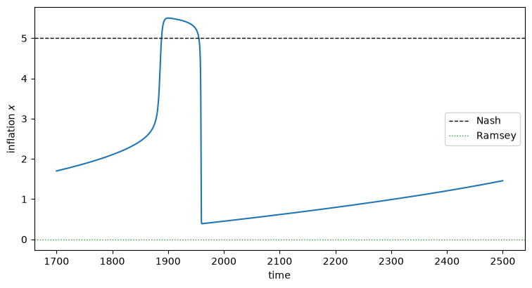
Fig. 105.3 Inflation oscillates between Nash and Ramsey along the learning cycle#
This is qualitatively different from the escapes of Adaptive Learning and Escape Dynamics.
There, disinflations were rare events, driven by unlikely sequences of shocks; between them the system sat at Nash.
Here the disinflations are a typical feature of the time series, produced by the mean dynamics themselves — a deterministic cycle that persists even as the gain shrinks to zero.
105.7. Escape dynamics and the direction of escape#
For priors that keep the self-confirming equilibrium stable, disinflations return to being rare escapes, exactly as in Adaptive Learning and Escape Dynamics.
The theory of large deviations (developed in the primer of Adaptive Learning and Escape Dynamics, and applied here via [Williams, 2019]) characterizes the most likely escape as the solution of a control problem: apply the least-cost perturbation to beliefs that pushes them a fixed distance from \(\bar\gamma\).
The instantaneous escape direction has a beautifully simple characterization: it is the eigenvector associated with the largest eigenvalue of the belief-innovation covariance \(Q(\bar\gamma, \bar P) = \hat V\) — the prior itself.
w, vecs = np.linalg.eigh(V_star)            # baseline prior V*
v_escape = vecs[:, np.argmax(w)]
v_escape = v_escape / np.linalg.norm(v_escape)

# scale the escape so the slope moves from -1 up to 0
t_star = 1.0 / v_escape[1]
terminal = γ_sce + t_star * v_escape

print(f"escape direction  ≈ {v_escape.round(3)}   (∝ [-u, 1])")
print(f"terminal beliefs  ≈ {terminal.round(2)}   (Belief 2 = [u, 0] = Ramsey)")
escape direction  ≈ [-0.981  0.195]   (∝ [-u, 1])
terminal beliefs  ≈ [4.98 0.  ]   (Belief 2 = [u, 0] = Ramsey)
For the baseline prior the escape direction is proportional to \((-u, 1)\), and it carries beliefs from Nash \((2u, -1)\) toward \((u, 0)\) — Belief 2, which supports the Ramsey outcome.
So an escape, when it happens, is a movement toward zero inflation.
Different priors bend the path and change the rate of escape — tightening the slope prior can even destabilize the equilibrium entirely (the cycles above), while tightening the intercept prior speeds escapes up — but the destination is always Ramsey.
105.8. Sims’s nonconvergence#
We can now resolve a puzzle noted in The Rise and Fall of U.S. Inflation.
The simulations of [Sims, 1988] and [Chung, 1990] start at the Nash self-confirming outcome, escape to low inflation, and then stay there, apparently indefinitely.
Those of [Sargent, 1999] and CWS instead escape and are then pulled back, again and again.
[Sargent and Williams, 2005] trace the difference to a single modeling choice: whether the government attributes the right amount of variance to its regression error.
When \(\sigma = \sigma_1\) — as in a self-confirming equilibrium, where the regression (105.2) and the truth (105.1) coincide — the government correctly decomposes the variation it sees.
Sims instead used \(\sigma \neq \sigma_1\) (and did not shrink the gain), which misallocates the observed variation and produces prolonged, perhaps permanent, departures from the self-confirming equilibrium.
The mechanism is visible in the Riccati equation (105.6) before we simulate anything.
A government that attributes too little variance to its regression error must attribute the variation it sees to something else, and the only thing else available is drift in its own coefficients.
So \(\sigma < \sigma_1\) inflates the steady-state \(P\), and \(P\) is what multiplies each forecast error in (105.5).
Understating the error variance therefore makes the government learn faster — which is precisely what weakens the pull of the mean dynamics.
def effective_gain(model, σ_govt, ε, λ=1.0):
    "Steady-state weight the filter puts on a single forecast error at the SCE."
    V = ε**2 * V_tighten_slope(λ, V_star)
    P = solve_riccati(V, M_sce, σ_govt)
    Φ = np.array([1.0, model.x(γ_sce)])
    return (P @ Φ)[0] / (σ_govt**2 + Φ @ P @ Φ)

ε_common = 0.0002
for σ_govt, tag in ((model.σ1, 'σ = σ1  (correct) '), (0.1, 'σ ≠ σ1  (Sims)   ')):
    print(f"{tag}: effective gain = {effective_gain(model, σ_govt, ε_common):.5f}")
σ = σ1  (correct) : effective gain = 0.00222
σ ≠ σ1  (Sims)   : effective gain = 0.05660
Understating the error variance multiplies the effective gain by more than twenty, even though the prior \(V\) and the scale \(\varepsilon\) are identical in the two runs.
Let’s now simulate the static model under both specifications, holding \(\varepsilon\) fixed so that the only difference is the variance the government attributes to its own regression error.
def simulate(model, σ_govt, ε, λ=1.0, T=3000, seed=0):
    "Static Kalman-filter learning; σ_govt is the government's assumed error std."
    rng = np.random.default_rng(seed)
    u, σ1, σ2 = model.u, model.σ1, model.σ2

    V = ε**2 * V_tighten_slope(λ, V_star)
    γ = γ_sce.copy()
    P = ε * np.linalg.inv(M_sce)
    infl = np.empty(T)

    for n in range(T):
        x = model.x(γ)
        w1, w2 = rng.standard_normal(2)
        π = x + σ2 * w2
        U = u - σ2 * w2 + σ1 * w1                 # truth uses σ1
        Φ = np.array([1.0, π])
        denom = σ_govt**2 + Φ @ P @ Φ
        γ = γ + (P @ Φ) / denom * (U - Φ @ γ)
        P = P - np.outer(P @ Φ, Φ @ P) / denom + V / σ_govt**2
        infl[n] = π
    return infl

T_sim, seeds = 6000, range(10)

def summarize(σ_govt):
    "Mean inflation and time near Ramsey, across seeds."
    paths = [simulate(model, σ_govt=σ_govt, ε=ε_common, T=T_sim, seed=s)
             for s in seeds]
    return (np.array([p.mean() for p in paths]),
            np.array([(p < 2).mean() for p in paths]))

mean_base, ramsey_base = summarize(model.σ1)
mean_sims, ramsey_sims = summarize(0.1)

print(f"{'seed':>4} | {'σ = σ1: mean π':>15} {'near Ramsey':>12}"
      f" | {'σ ≠ σ1: mean π':>15} {'near Ramsey':>12}")
for s in seeds:
    print(f"{s:>4} | {mean_base[s]:>15.2f} {ramsey_base[s]:>11.0%}"
          f" | {mean_sims[s]:>15.2f} {ramsey_sims[s]:>11.0%}")
print(f"\nnever escaped in {T_sim} periods:  "
      f"σ = σ1: {np.sum(ramsey_base < 0.01)}/{len(seeds)} paths,   "
      f"σ ≠ σ1: {np.sum(ramsey_sims < 0.01)}/{len(seeds)} paths")
seed |  σ = σ1: mean π  near Ramsey |  σ ≠ σ1: mean π  near Ramsey
   0 |            4.99          0% |            2.26         58%
   1 |            5.04          0% |            2.24         58%
   2 |            1.16         79% |            1.70         69%
   3 |            1.10         80% |            2.09         61%
   4 |            4.39         10% |            1.58         73%
   5 |            5.02          0% |            2.24         58%
   6 |            0.43         94% |            1.71         69%
   7 |            0.50         92% |            2.12         61%
   8 |            5.02          0% |            1.99         62%
   9 |            1.82         64% |            1.96         64%

never escaped in 6000 periods:  σ = σ1: 4/10 paths,   σ ≠ σ1: 0/10 paths
The two columns behave quite differently, and the difference is about how often the economy leaves Nash rather than about where it goes when it does.
With the correct error variance, an escape is a genuinely rare event: several of the sample paths sit at the Nash rate for six thousand periods without ever escaping at all, and the rest escape at some point and are held near Ramsey afterwards.
With Sims’s misallocation, every path escapes, and every one of them spends most of its time near Ramsey.
Three seeds make the point without any cherry-picking: seed 0 never escapes, seed 4 escapes repeatedly and is pulled back each time, and seed 6 escapes and stays away for a long spell.
show = (0, 4, 6)

fig, axes = plt.subplots(2, 1, figsize=(9.5, 7), sharex=True, sharey=True)
for s in show:
    axes[0].plot(simulate(model, σ_govt=model.σ1, ε=ε_common, T=T_sim, seed=s),
                 lw=0.5, label=f'seed {s}')
    axes[1].plot(simulate(model, σ_govt=0.1, ε=ε_common, T=T_sim, seed=s),
                 lw=0.5, label=f'seed {s}')
for ax, title in zip(axes, [r'$\sigma = \sigma_1$ (correct): escapes are rare events',
                            r'$\sigma \neq \sigma_1$ (Sims): every path escapes and lingers']):
    ax.axhline(model.u, color='k', ls='--', lw=1)
    ax.axhline(0, color='C2', ls=':', lw=1)
    ax.set_ylabel('inflation')
    ax.set_title(title)
    ax.legend(frameon=False, fontsize=8, ncol=3, loc='lower right')
axes[1].set_xlabel('$n$')
plt.tight_layout()
plt.show()
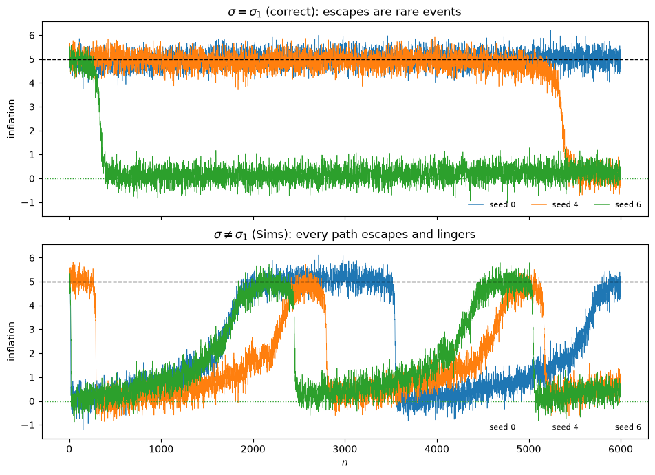
Fig. 105.4 Escapes are rare under the correct error variance and pervasive under Sims’s misallocation#
With the correct error variance the mean dynamics dominate: the economy sits at Nash, and only an unusual run of shocks dislodges it — the rare-escape picture of Adaptive Learning and Escape Dynamics and Escaping Nash Inflation.
With Sims’s misallocation the government learns too fast for the mean dynamics to hold it, so it escapes almost immediately and behaves as if it had permanently learned a good-enough version of the natural-rate hypothesis.
As [Sargent and Williams, 2005] put it, one can read the difference in two equivalent ways: either Sims allowed too much parameter drift to permit convergence, or he did not let the government attribute enough variation to its regression error.
105.9. Conclusion#
Free parameters are dangerous, as Arthur Goldberger and Robert Lucas warned.
This lecture’s government carries free parameters in the covariance matrix \(V\) of the drift in its beliefs.
But those parameters buy something: the empirical sequel [Sargent et al., 2006] shows that estimating \(V\) from post-war U.S. data lets the model reverse-engineer a sequence of policy makers’ evolving subjective models of the Phillips curve that rationalize the actual rise and fall of American inflation — the vindication story of The Rise and Fall of U.S. Inflation, made quantitative.
Related evidence that the covariance of coefficient drift has itself moved over time appears in [Cogley and Sargent, 2005].
105.9.1. Are the estimated beliefs realistic?#
That empirical success came with a challenge that is really a challenge about the prior.
To fit the data, [Sargent et al., 2006] estimated a large drift covariance \(V\) — a government so open to new data that its beliefs about the monetary transmission mechanism lurch from month to month.
[Primiceri, 2006], Christopher Sims, and, candidly, [Sargent, 2008] in his presidential address, objected that such volatile beliefs are unrealistic: the imputed government forecasts unemployment poorly and holds views no real central bank would.
[Carboni and Ellison, 2009] answer the objection by disciplining the prior with data the Federal Reserve actually produced.
They re-estimate the model subject to the requirement that its beliefs reproduce the unemployment forecasts published in the Fed’s Greenbook — imposing on the learning model a cross-equation restriction of the kind familiar from rational-expectations econometrics.
Imposing it shrinks the estimated \(V\) by orders of magnitude and removes the wild belief swings, yet leaves the low-frequency conquest story intact: a stable evolution of Federal Reserve beliefs still explains the rise and fall of inflation.
The volatile beliefs, it turns out, were doing nothing but overfitting the high-frequency wiggles that [Sargent, 1999] never set out to explain.
The moral for this lecture is direct: the prior \(V\) is not a nuisance parameter to be maximized over freely — it is an economic object, and pinning it down with independent evidence on what policy makers actually believed is what makes the vindication story credible.
The broader message is that how an adaptive government learns — the prior it brings to the drift in its own beliefs — is not a technical detail.
It determines whether the economy converges to Nash, cycles between Nash and Ramsey, or escapes to Ramsey and stays there.
The Lost Conquest: Fed Policy in the 2020s carries these same tools — constant-gain learning, an anticipated-utility Phelps problem, and a self-confirming equilibrium — into the present, to rationalize the Federal Reserve’s response to the inflation of the 2020s.
Drifts and Volatilities then closes the suite by putting the whole account to an empirical test, fitting a drifting-coefficient, stochastic-volatility VAR to post-war data and asking how much of the Great Inflation was drifting beliefs and how much was simply bad luck.
105.10. Exercises#
Exercise 105.1
The learning cycle above tightened the prior on the slope coefficient.
Tightening the prior on the intercept coefficient instead — using
— does not destabilize the self-confirming equilibrium.
Verify this by plotting the maximum real part of the eigenvalues of \(\bar P(\lambda)\,\partial\bar g/\partial\gamma\) against \(\lambda\) for this intercept-tightening family, and confirm it stays negative.
Solution
def V_tighten_intercept(λ, V_star):
    V = V_star.copy()
    V[0, 0] = λ * V_star[0, 0]
    V[0, 1] = V[1, 0] = np.sqrt(λ) * V_star[0, 1]
    return V

max_re_int = []
for λ in λ_grid:
    V = ε**2 * V_tighten_intercept(λ, V_star)
    P = solve_riccati(V, M_sce, model.σ)
    max_re_int.append(np.linalg.eigvals(P @ J).real.max())

fig, ax = plt.subplots(figsize=(8, 4.5))
ax.plot(λ_grid, max_re_int, label='tighten intercept')
ax.plot(λ_grid, max_re, ls='--', label='tighten slope (for comparison)')
ax.axhline(0, color='k', lw=0.8)
ax.set_xlabel(r'$\lambda$')
ax.set_ylabel('max real part of eigenvalue')
ax.set_title('Stability under a tighter intercept prior')
ax.legend()
plt.show()
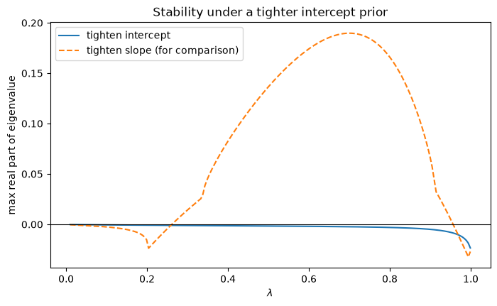
Tightening the intercept prior keeps the maximum real part negative for all \(\lambda\): the self-confirming equilibrium stays stable, so there is no learning cycle.
As [Sargent and Williams, 2005] show, this prior does still change the escape dynamics — it speeds escapes up — but it does not overturn the mean dynamics.
Exercise 105.2
The instantaneous escape direction is the dominant eigenvector of the prior covariance \(\hat V\).
Confirm that this direction is robust to the overall scale of the prior but sensitive to its shape.
Compute the escape direction (and the implied terminal beliefs) for the baseline prior \(V^*\) and for the slope-tightened prior \(V(\lambda = 0.5)\), and compare where each sends the government’s beliefs.
Solution
def escape_terminal(V):
    w, vecs = np.linalg.eigh(V)
    v = vecs[:, np.argmax(w)]
    v = v / np.linalg.norm(v)
    if v[1] < 0:                      # orient toward increasing slope
        v = -v
    return γ_sce + (1.0 / v[1]) * v, v

for name, V in [("baseline V*", V_star),
                ("slope-tightened V(0.5)", V_tighten_slope(0.5, V_star))]:
    term, v = escape_terminal(V)
    print(f"{name:24s}: direction {v.round(3)}, terminal {term.round(2)}")
baseline V*             : direction [-0.981  0.195], terminal [4.98 0.  ]
slope-tightened V(0.5)  : direction [-0.99  0.14], terminal [2.9 0. ]
Both priors send beliefs toward a terminal point with slope \(0\) — the Ramsey belief — but along different directions, and the intercepts they arrive at differ considerably: the slope-tightened prior lands at an intercept a little over half the baseline’s.
The destination is robust in the sense that matters for policy: slope \(0\) means the government perceives no exploitable tradeoff, and (105.3) then sets inflation to zero whatever the intercept.
The route, and where along the Ramsey line the escape terminates, depend on the shape of the prior.