22. Exponential Family and Maximum Entropy#
22.1. Overview#
This lecture and its sequel Information Projections describe some elements of information geometry, a body of work that studies families of probability distributions with tools from convex analysis and differential geometry.
We use information geometry to describe the exponential family of probability distributions.
The exponential family includes the Bernoulli, Poisson, normal, gamma, and Beta distributions.
A convex function, the log-partition function, generates
two systems of coordinates for the members of a family, called natural parameters and expectation parameters;
the means and covariances of the family’s sufficient statistics;
the Fisher information matrix;
the entropy of each member, through a Legendre transform, when the family’s base measure is constant; and
the Kullback–Leibler (KL) divergence between any two members, through a Bregman divergence.
Members of the exponential family answer a question posed by Jaynes [1957]: which probability distribution expresses the least information, as measured by Shannon’s entropy, among all distributions that have given means of some statistics?
A special case characterizes the normal distribution: among all densities on the real line with a given mean and variance, the normal density has the largest entropy.
Economists already use several of these tools under other names.
The log-partition function and its Legendre transform are related in the same way as a profit function and a production function.
The formula for the derivative of the log-partition function is a version of Hotelling’s lemma.
The inclusive value of the multinomial logit model of discrete choice is a log-partition function.
Up to a constant, it is the expected utility of the best alternative.
Its Legendre transform is minus an entropy.
The sequel Information Projections uses these tools to study projections of probability distributions onto families of distributions, with applications to maximum likelihood, robust control, the updating of input–output tables, and optimal transport.
The lecture builds on Statistical Divergence Measures, which describes entropy, cross-entropy, and KL divergence; we use its notation.
Maximum Likelihood Estimation and Multivariate Normal Distribution provide additional background.
Amari and Nagaoka [2000], Nielsen [2020], and chapters 2, 8, 11, and 12 of Cover and Thomas [2006] treat the material of this lecture and its sequel.
We use the following imports.
import numpy as np
import matplotlib.pyplot as plt
from scipy import integrate
from scipy.optimize import brentq
from scipy.special import logsumexp, digamma, polygamma, gammaln
from scipy.stats import norm, poisson, laplace, logistic, uniform, chi2
from scipy.stats import gamma as gamma_dist
22.2. Coordinates matter#
We usually describe a normal distribution by its mean \(\mu\) and standard deviation \(\sigma\).
The pair \((\mu, \sigma)\) is a point in a half-plane, but the ordinary distance between two such points says little about how hard it is to tell the two distributions apart from data.
Consider four normal distributions:
\(A = N(0, 0.2^2)\) and \(B = N(1, 0.2^2)\), and
\(C = N(0, 2^2)\) and \(D = N(1, 2^2)\).
In the \((\mu, \sigma)\) half-plane, \(A\) is as far from \(B\) as \(C\) is from \(D\).
But \(A\) and \(B\) barely overlap, while \(C\) and \(D\) overlap heavily.
The KL divergence between two normal distributions with a common standard deviation \(\sigma\) is \((\mu_1 - \mu_2)^2 / (2 \sigma^2)\), which is \(12.5\) for \(A\) and \(B\) and \(0.125\) for \(C\) and \(D\).
x = np.linspace(-6, 7, 1000)
fig, axes = plt.subplots(1, 2, figsize=(10, 3.5))
for ax, σ, names in zip(axes, (0.2, 2.0), (("A", "B"), ("C", "D"))):
    for μ, name in zip((0.0, 1.0), names):
        ax.plot(x, norm.pdf(x, μ, σ), lw=2, label=f"{name}: N({μ:g}, {σ:g}²)")
    ax.set_title(rf"$\sigma = {σ:g}$, KL = {1 / (2 * σ**2):.3g}")
    ax.set_xlabel("$x$")
    ax.legend()
plt.tight_layout()
plt.show()
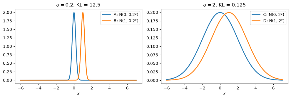
Fig. 22.1 Equal parameter distances, unequal KL divergences#
A geometry of probability distributions should measure distances by how distinguishable distributions are.
For the exponential family, one convex function generates such a geometry.
22.3. Maximum entropy#
22.3.1. A die#
Edwin Jaynes proposed the maximum entropy principle [Jaynes, 1957] and illustrated it in his 1962 Brandeis lectures with the following problem, now known as the Brandeis dice problem [Jaynes, 1963].
A die has faces \(x \in \{1, 2, \ldots, 6\}\).
We are told only that the average number of spots is \(4.5\), rather than the \(3.5\) of a fair die.
Which probability distribution \(p = (p_1, \ldots, p_6)\) should we assign to the faces?
Many distributions have mean \(4.5\).
Jaynes proposed choosing the one that is “maximally noncommittal with regard to missing information” [Jaynes, 1957], which he took to mean the one that maximizes Shannon’s entropy
subject to \(\sum_x p(x) = 1\) and \(\sum_x x \, p(x) = 4.5\).
22.3.2. The solution is an exponential family#
Let’s solve a more general version of this problem.
Let \(t(x) = (t_1(x), \ldots, t_d(x))\) be a vector of functions of the outcome \(x\), which takes values in a finite set.
We seek the distribution \(p\) that maximizes \(H(p)\) subject to the moment conditions
for a given vector \(c\), and \(\sum_x p(x) = 1\).
Attach a vector of Lagrange multipliers \(\theta\) to (22.1).
The first-order condition for \(p(x)\) is \(-\log p(x) - 1 + \theta \cdot t(x) - \nu = 0\), where \(\nu\) is the multiplier on \(\sum_x p(x) = 1\).
The solution has the form
where \(\theta\) satisfies (22.1).
The function \(F\) makes the probabilities sum to one.
Such a \(\theta\) exists if and only if \(c\) lies in the relative interior of the convex hull of the points \(t(x)\), that is, in its interior as a subset of the smallest affine subspace that contains it; for the die below, if and only if \(1 < c < 6\).
When \(c\) lies on the relative boundary, as for a die whose mean is \(6\), a maximizing distribution still exists.
It puts zero probability on some outcomes, and it lies outside the family, as a limit of members whose \(\theta\) diverges.
A family of distributions of the form (22.2) is called an exponential family.
The Lagrange multipliers \(\theta\) are its natural parameters, and \(t\) is its sufficient statistic.
To confirm that (22.2) is a maximum, let \(p\) be any distribution that satisfies (22.1), and let \(p^*\) be the member of the exponential family that satisfies it.
Because \(\log p^*(x) = \theta \cdot t(x) - F(\theta)\) is an affine function of \(t(x)\), and \(p\) and \(p^*\) assign the same mean \(c\) to \(t\),
We read \(D_{KL}(p \| q) = \sum_x p(x) \log (p(x) / q(x))\) as “the KL divergence of \(p\) from \(q\).”
Therefore
with equality only if \(p = p^*\).
Among all distributions that satisfy the moment conditions, the member of the exponential family has the largest entropy, and the entropy shortfall of any other distribution equals its KL divergence from that member.
The sequel Information Projections shows that (22.3) is an instance of a Pythagorean theorem.
For Jaynes’s die, \(t(x) = x\) and \(\theta\) is a scalar.
The function tilt below computes the exponential tilt of a base distribution \(q\): the distribution proportional to \(q(x) \exp(\theta \, t(x))\) for a statistic \(t\).
For the maximum entropy problem, \(q\) is uniform, and the result is (22.2).
The second function finds the \(\theta\) that delivers a given mean.
def tilt(q, t, θ):
    """The distribution proportional to q(x) exp(θ t(x))."""
    log_w = np.log(q) + θ * t
    return np.exp(log_w - logsumexp(log_w))


def match_mean(q, t, c):
    """Find θ such that the tilted distribution has mean c."""
    θ = brentq(lambda θ: tilt(q, t, θ) @ t - c, -50, 50)
    return θ, tilt(q, t, θ)


def entropy(p):
    return -p @ np.log(p)


def kl(p, q):
    return p @ np.log(p / q)


faces = np.arange(1, 7)
uniform_die = np.full(6, 1 / 6)
θ_die, p_die = match_mean(uniform_die, faces, 4.5)
print(f"θ = {θ_die:.4f}")
print("maximum entropy distribution:", np.round(p_die, 4))
print(f"entropy = {entropy(p_die):.4f}, compared with log 6 = {np.log(6):.4f}")
θ = 0.3710
maximum entropy distribution: [0.0544 0.0788 0.1142 0.1654 0.2398 0.3475]
entropy = 1.6136, compared with log 6 = 1.7918
The probabilities rise geometrically, by the factor \(e^{\theta}\) from one face to the next.
Let’s check (22.3) by drawing other distributions with mean \(4.5\).
We construct them by moving away from \(p^*\) in directions that preserve both the total probability and the mean.
rng = np.random.default_rng(0)

# directions orthogonal to (1, ..., 1) and to (1, 2, ..., 6)
constraints = np.vstack([np.ones(6), faces])
null_space = np.linalg.svd(constraints)[2][2:].T

print(" H(p*) - H(p)    KL(p || p*)")
for _ in range(5):
    while True:
        p = p_die + null_space @ rng.normal(scale=0.05, size=4)
        if np.all(p > 0):
            break
    print(f"{entropy(p_die) - entropy(p):12.6f} {kl(p, p_die):14.6f}")
 H(p*) - H(p)    KL(p || p*)
    0.004630       0.004630
    0.042067       0.042067
    0.028720       0.028720
    0.116931       0.116931
    0.018324       0.018324
The figure shows the maximum entropy distributions for several means.
fig, ax = plt.subplots()
for c in (2.5, 3.5, 4.5, 5.5):
    θ, p = match_mean(uniform_die, faces, c)
    ax.plot(faces, p, "o-", label=rf"mean {c}, $\theta$ = {θ:.2f}")
ax.set_xlabel("face")
ax.set_ylabel("probability")
ax.legend()
plt.show()
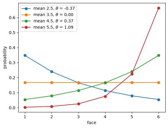
Fig. 22.2 Maximum entropy die distributions by mean#
22.3.3. The normal distribution#
Now let the outcome \(x\) be a real number, and constrain its mean and its second moment:
For a density \(p\) on the real line, the differential entropy is \(H(p) = -\int p(x) \log p(x) \, dx\).
The argument that led to (22.2) now says that the density with the largest entropy has the form
which is integrable only if \(\theta_2 < 0\).
Completing the square shows that this is the normal density with \(\theta_1 = \mu / \sigma^2\) and \(\theta_2 = -1/(2\sigma^2)\).
The argument that delivered (22.3) goes through with sums replaced by integrals, so that every density \(p\) with mean \(\mu\) and variance \(\sigma^2\) satisfies
where \(\varphi\) is the \(N(\mu, \sigma^2)\) density.
Among all densities on the real line with a given mean and variance, the normal density has the largest entropy.
Its entropy is \(H(\varphi) = \frac{1}{2} \log(2 \pi e \sigma^2)\).
Unlike the entropy of a discrete distribution, differential entropy can be negative, and it changes when we change the units in which \(x\) is measured; the gap (22.4) is a KL divergence and does neither.
We check (22.4) for several densities with mean zero and variance one.
We compute the entropies with SciPy’s formulas and the KL divergences by numerical integration.
φ = norm(0, 1)
alternatives = {
    "uniform": uniform(-np.sqrt(3), 2 * np.sqrt(3)),
    "Laplace": laplace(0, 1 / np.sqrt(2)),
    "logistic": logistic(0, np.sqrt(3) / np.pi),
}

print(f"entropy of N(0, 1): {φ.entropy():.4f}\n")
print(f"{'distribution':12} {'variance':>8} {'entropy':>8} "
      f"{'H(φ) - H(p)':>12} {'KL(p || φ)':>11}")
for name, dist in alternatives.items():
    a, b = dist.support()
    a, b = max(a, -30), min(b, 30)
    kl_p_φ = integrate.quad(
        lambda x: dist.pdf(x) * (dist.logpdf(x) - φ.logpdf(x)), a, b,
        limit=200)[0]
    print(f"{name:12} {dist.var():8.4f} {dist.entropy():8.4f} "
          f"{φ.entropy() - dist.entropy():12.4f} {kl_p_φ:11.4f}")
entropy of N(0, 1): 1.4189

distribution variance  entropy  H(φ) - H(p)  KL(p || φ)
uniform        1.0000   1.2425       0.1765      0.1765
Laplace        1.0000   1.3466       0.0724      0.0724
logistic       1.0000   1.4046       0.0144      0.0144
We can also watch the normal distribution emerge from a discrete maximum entropy problem.
Put the outcome on a fine grid of points and impose the two moment conditions.
The function below finds the natural parameters by Newton’s method, using two facts that we prove below: the gradient of \(F\) is the vector of means of \(t\), and the Hessian of \(F\) is the covariance matrix of \(t\).
def maxent(q, T, c, tol=1e-12, max_iter=100):
    """
    Maximize entropy relative to q subject to E[T] = c.

    T is an m × d array whose rows are t(x).  Returns θ and the
    distribution proportional to q(x) exp(θ · t(x)).  The iterations
    converge only if c is in the interior of the convex hull of the
    rows of T.
    """
    def tilted(θ):
        log_w = np.log(q) + T @ θ
        return np.exp(log_w - logsumexp(log_w))

    θ = np.zeros(T.shape[1])
    for _ in range(max_iter):
        p = tilted(θ)
        mean = p @ T
        cov = (T - mean).T @ ((T - mean) * p[:, None])
        step = np.linalg.solve(cov, c - mean)
        θ = θ + step
        if np.max(np.abs(step)) < tol:
            break
    else:
        raise RuntimeError("no convergence: is c inside the hull of t(x)?")
    return θ, tilted(θ)


μ_grid, σ_grid = 1.0, 1.2
grid = np.linspace(-6, 6, 241)
spacing = grid[1] - grid[0]
T_grid = np.column_stack([grid, grid**2])
θ_grid, p_grid = maxent(np.full(grid.size, 1 / grid.size), T_grid,
                        c=np.array([μ_grid, μ_grid**2 + σ_grid**2]))
print(f"θ = {np.round(θ_grid, 4)}")
print(f"(μ/σ², -1/(2σ²)) = "
      f"{np.round([μ_grid / σ_grid**2, -1 / (2 * σ_grid**2)], 4)}")
θ = [ 0.6943 -0.3471]
(μ/σ², -1/(2σ²)) = [ 0.6944 -0.3472]
fig, ax = plt.subplots()
ax.plot(grid, p_grid / spacing, lw=4, alpha=0.4,
        label="maximum entropy on a grid")
ax.plot(grid, norm.pdf(grid, μ_grid, σ_grid), "k--", lw=1,
        label=f"N({μ_grid:g}, {σ_grid:g}²)")
ax.set_xlabel("$x$")
ax.legend(loc="upper right")
plt.show()
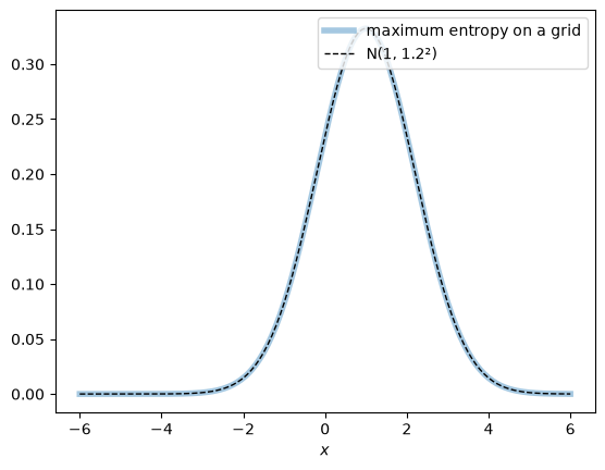
Fig. 22.3 Grid maximum entropy matches the normal#
22.3.4. Other moment conditions#
Different moment conditions produce different families.
outcomes |
constrained means |
maximum entropy distribution |
|---|---|---|
\(\{1, \ldots, m\}\) |
none |
uniform |
\(\{0, 1, 2, \ldots\}\) |
\(E[X]\) |
geometric |
\([a, b]\) |
none |
uniform |
\([0, \infty)\) |
\(E[X]\) |
exponential |
\((0, \infty)\) |
\(E[X]\), \(E[\log X]\) |
gamma |
\((0, \infty)\) |
\(E[\log X]\), \(E[(\log X)^2]\) |
lognormal |
\((0, 1)\) |
\(E[\log X]\), \(E[\log(1 - X)]\) |
Beta |
\(\mathbb{R}\) |
\(E[\lvert X \rvert]\) |
Laplace |
\(\mathbb{R}\) |
\(E[X]\), \(E[X^2]\) |
normal |
\(\mathbb{R}^m\) |
\(E[X]\), \(E[X X^\top]\) |
multivariate normal |
The last row implies that, among all densities on \(\mathbb{R}^m\) with a given mean vector and covariance matrix \(\Sigma\), the multivariate normal density has the largest entropy, \(\frac{1}{2} \log \det(2 \pi e \Sigma)\).
The lognormal row is the normal row applied to \(\log X\): a density on \((0, \infty)\) proportional to \(\exp(\theta_1 \log x + \theta_2 (\log x)^2)\) is a lognormal density.
Exercise 22.1 asks you to work out the gamma case.
22.4. The exponential family#
22.4.1. Definition#
A family of densities (or probability mass functions) is an exponential family if it can be written as
with the integral replaced by a sum when \(x\) is discrete, and where
\(t(x) \in \mathbb{R}^d\) is the sufficient statistic,
\(\theta \in \mathbb{R}^d\) is the natural parameter,
\(h(x) \geq 0\) is the base measure, and
\(F(\theta)\) is the log-partition function, also called the cumulant function.
The natural parameters range over the set \(\Theta\) of \(\theta\) for which the integral defining \(F\) is finite.
In the maximum entropy problem above, \(h\) is constant; in the function tilt, the base distribution \(q\) is the base measure \(h\).
A nonconstant \(h\) arises when we maximize entropy relative to a base distribution that is not uniform, a problem that Information Projections takes up.
We assume that the representation is minimal: no nontrivial linear combination \(a \cdot t(x)\) is constant on the set where \(h(x) > 0\).
Then different \(\theta\)’s give different distributions.
We also assume that \(\Theta\) is an open set, as it is for every family in this lecture.
Here are some familiar families written this way.
family |
\(t(x)\) |
\(\theta\) |
\(F(\theta)\) |
|---|---|---|---|
Bernoulli(\(\pi\)) |
\(x\) |
\(\log \frac{\pi}{1 - \pi}\) |
\(\log(1 + e^{\theta})\) |
Poisson(\(\lambda\)) |
\(x\) |
\(\log \lambda\) |
\(e^{\theta}\) |
exponential(\(\lambda\)) |
\(x\) |
\(-\lambda\) |
\(-\log(-\theta)\) |
\(N(\mu, \sigma^2)\) |
\((x, x^2)\) |
\(\left(\frac{\mu}{\sigma^2}, -\frac{1}{2\sigma^2}\right)\) |
\(-\frac{\theta_1^2}{4 \theta_2} + \frac{1}{2}\log\left(-\frac{\pi}{\theta_2}\right)\) |
Beta(\(a\), \(b\)) |
\((\log x, \log(1 - x))\) |
\((a - 1, b - 1)\) |
\(\log B(\theta_1 + 1, \theta_2 + 1)\) |
categorical(\(\pi\)) |
\((1_{x = 1}, \ldots, 1_{x = K - 1})\) |
\(\left(\log \frac{\pi_k}{\pi_K}\right)_{k < K}\) |
\(\log\left(1 + \sum_{k < K} e^{\theta_k}\right)\) |
In every row \(h(x) = 1\), except the Poisson row, where \(h(x) = 1/x!\).
In the Bernoulli and categorical rows \(\pi\) is a probability or a vector of probabilities; in the normal row it is \(3.14159\ldots\).
In the Beta row, \(B\) is the beta function.
The categorical family on \(\{1, \ldots, K\}\) uses only \(K - 1\) indicators, because all \(K\) indicators sum to one; with all \(K\), the representation would not be minimal.
The multivariate normal \(N(\mu, \Sigma)\) is an exponential family with \(t(x) = (x, x x^\top)\) and natural parameters \((\Sigma^{-1}\mu, -\frac{1}{2}\Sigma^{-1})\), where the pairing is \(\theta \cdot t(x) = \theta_1 \cdot x + x^\top \Theta_2 x\) with \(\Theta_2\) a symmetric matrix.
Because \(x_i x_j = x_j x_i\), a minimal representation keeps only the entries of \(x x^\top\) on and above the diagonal.
A family of the form (22.5) contains every normalized geometric mixture of two of its members: the distribution proportional to \(p(x; \theta_0)^{1 - a} p(x; \theta_1)^a\) has natural parameter \((1 - a)\theta_0 + a \theta_1\), for every \(a \in [0, 1]\) and for any other \(a\) for which that parameter lies in \(\Theta\).
The sequel Information Projections builds a geometry on this fact.
The log-partition function determines everything else.
22.4.2. The log-partition function generates moments#
Differentiate \(F(\theta) = \log \int h(x) \exp(\theta \cdot t(x)) \, dx\):
Differentiating again gives
The function \(F\) is convex because a covariance matrix is positive semidefinite; minimality makes \(\operatorname{Cov}_\theta[t(X)]\) positive definite, so \(F\) is strictly convex.
More generally, \(\log E_\theta \exp(s \cdot t(X)) = F(\theta + s) - F(\theta)\), so the derivatives of \(F\) are the cumulants of \(t(X)\).
Let’s verify (22.6) and (22.7) for the Poisson and normal families, comparing finite-difference derivatives of \(F\) with moments computed by summation and integration.
def F_poisson(θ):
    return np.exp(θ)


def F_normal(θ):
    θ1, θ2 = θ
    return -θ1**2 / (4 * θ2) + 0.5 * np.log(-np.pi / θ2)


def normal_θ(μ, σ):
    return np.array([μ / σ**2, -1 / (2 * σ**2)])


def gradient(F, θ, h=1e-5):
    θ = np.atleast_1d(np.asarray(θ, dtype=float))
    e = np.eye(θ.size) * h
    return np.array([np.squeeze(F(θ + e[i]) - F(θ - e[i])) / (2 * h)
                     for i in range(θ.size)])


def hessian(F, θ, h=1e-4):
    θ = np.atleast_1d(np.asarray(θ, dtype=float))
    e = np.eye(θ.size) * h
    return np.array([(gradient(F, θ + e[i]) - gradient(F, θ - e[i])) / (2 * h)
                     for i in range(θ.size)])


λ = 3.0
k = np.arange(100)
pk = poisson.pmf(k, λ)
print("Poisson:  F'(θ), F''(θ) =",
      np.round([gradient(F_poisson, np.log(λ))[0],
                hessian(F_poisson, np.log(λ))[0, 0]], 6),
      "  mean, variance =", np.round([pk @ k, pk @ k**2 - (pk @ k)**2], 6))

μ, σ = 0.5, 1.2
moments = [integrate.quad(lambda x: x**j * norm.pdf(x, μ, σ), -15, 15)[0]
           for j in range(1, 5)]
mean_t = np.array(moments[:2])
cov_t = np.array([[moments[1] - moments[0]**2,
                   moments[2] - moments[0] * moments[1]],
                  [moments[2] - moments[0] * moments[1],
                   moments[3] - moments[1]**2]])
print("\nnormal:  ∇F(θ) =", np.round(gradient(F_normal, normal_θ(μ, σ)), 6),
      "  E[t] =", np.round(mean_t, 6))
print("∇²F(θ) =\n", np.round(hessian(F_normal, normal_θ(μ, σ)), 4))
print("Cov[t] =\n", np.round(cov_t, 4))
Poisson:  F'(θ), F''(θ) = [3. 3.]   mean, variance = [3. 3.]

normal:  ∇F(θ) = [0.5  1.69]   E[t] = [0.5  1.69]
∇²F(θ) =
 [[1.44   1.44  ]
 [1.44   5.5872]]
Cov[t] =
 [[1.44   1.44  ]
 [1.44   5.5872]]
22.5. Two coordinate systems#
22.5.1. Expectation parameters#
By (22.6), the map \(\theta \mapsto \eta = \nabla F(\theta) = E_\theta[t(X)]\) sends each natural parameter to the vector of means of the sufficient statistic.
This map is one-to-one because \(F\) is strictly convex.
For the families in this lecture, its range is the interior of the convex hull of the values that \(t(X)\) can take: a Bernoulli mean lies strictly between \(0\) and \(1\), a Poisson mean is positive, and so on.
We can label each member of the family either by its natural parameter \(\theta\) or by its expectation parameter \(\eta\).
For the normal family, \(\eta = (\mu, \mu^2 + \sigma^2)\); for the Poisson family, \(\eta = \lambda\); for the Bernoulli family, \(\eta = \pi\).
The maximum entropy problem fixes the expectation parameters \(\eta = c\); its solution delivers the natural parameters \(\theta\).
22.5.2. Legendre duality#
The map from \(\eta\) back to \(\theta\) is the gradient of another convex function.
The convex conjugate, or Legendre transform, of \(F\) is
For \(\eta\) in the range of \(\nabla F\), the supremum is attained where \(\eta = \nabla F(\theta)\), so
and, by the envelope theorem, \(\nabla F^*(\eta) = \theta\).
The two gradient maps \(\nabla F\) and \(\nabla F^*\) are inverse functions, and their Jacobians are inverse matrices:
Because \(F\) is convex, applying the transform twice returns \(F\):
Economists use the same duality between a profit function and a production function.
In Pareto Distributions and Aggregate Production Functions, the industry profit function is \(\Pi(p) = \max_X \{ f(X) - p \cdot X \}\), where \(X\) is a vector of inputs, \(p\) is the vector of their prices, and \(f\) is the aggregate production function (which that lecture calls \(F\)).
Writing \(\theta = -p\) gives \(\Pi(-\theta) = \max_X \{ \theta \cdot X - (-f(X)) \}\), which has the same form as the last display.
The dictionary is
log-partition function \(F\) \(\leftrightarrow\) profit function \(\Pi\),
natural parameters \(\theta\) \(\leftrightarrow\) minus input prices \(-p\),
expectation parameters \(\eta\) \(\leftrightarrow\) input quantities \(X\), and
conjugate \(F^*\) \(\leftrightarrow\) minus the production function \(-f\).
Hotelling’s lemma, \(\partial \Pi / \partial p_i = -X_i\), is the counterpart of \(\nabla F(\theta) = \eta\), and recovering the production function from the profit function is the counterpart of recovering \(F^*\) from \(F\).
22.5.3. The conjugate is negative entropy#
Evaluate \(\log p(x; \theta) = \log h(x) + \theta \cdot t(x) - F(\theta)\) at a draw \(X\) from \(p(\cdot; \theta)\) and take expectations.
Using (22.9),
So when \(h(x) = 1\) wherever \(p(x; \theta) > 0\),
and the conjugate of the log-partition function is the negative of the entropy, expressed as a function of the expectation parameters.
In general, \(H(p(\cdot; \theta)) = -F^*(\eta) - E_\theta \log h(X)\).
Exercise 22.2 works out the Poisson case, where \(h(x) = 1/x!\).
For the Bernoulli family, \(h = 1\), \(F(\theta) = \log(1 + e^\theta)\), and \(F^*(\eta) = \eta \log \eta + (1 - \eta) \log (1 - \eta)\).
In the left panel of the figure below, the tangent line to \(F\) with slope \(\eta\) meets the vertical axis at \(-F^*(\eta)\).
In the right panel, the tangent line to \(F^*\) at \(\eta\) has slope \(\theta\).
def F_bern(θ):
    return np.log1p(np.exp(θ))


def F_star_bern(η):
    return η * np.log(η) + (1 - η) * np.log(1 - η)


θ0 = 2.0
η0 = 1 / (1 + np.exp(-θ0))

θ_vals = np.linspace(-4, 4, 200)
η_vals = np.linspace(0.001, 0.999, 200)

fig, axes = plt.subplots(1, 2, figsize=(10, 4))
ax = axes[0]
ax.plot(θ_vals, F_bern(θ_vals), lw=2, label=r"$F(\theta)$")
ax.plot(θ_vals, -F_star_bern(η0) + η0 * θ_vals, "--",
        label=rf"tangent line with slope $\eta$ = {η0:.2f}")
ax.plot([0], [-F_star_bern(η0)], "ko")
ax.annotate(r"$-F^*(\eta)$", (0, -F_star_bern(η0)),
            xytext=(8, -14), textcoords="offset points")
ax.plot([θ0], [F_bern(θ0)], "o", color="C1")
ax.axvline(0, color="0.7", lw=0.8)
ax.set_xlabel(r"$\theta$")
ax.legend()

ax = axes[1]
ax.plot(η_vals, F_star_bern(η_vals), lw=2, label=r"$F^*(\eta) = -H$")
ax.plot(η_vals, F_star_bern(η0) + θ0 * (η_vals - η0), "--",
        label=rf"tangent line with slope $\theta$ = {θ0:.2f}")
ax.plot([η0], [F_star_bern(η0)], "o", color="C1")
ax.set_xlabel(r"$\eta$")
ax.legend()
plt.tight_layout()
plt.show()
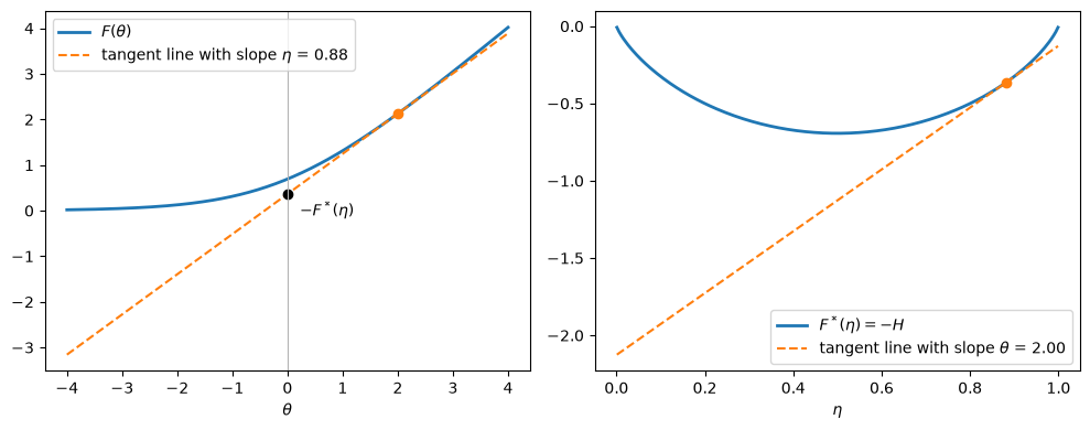
Fig. 22.4 Bernoulli log-partition function and its conjugate#
The Lagrange multipliers of the maximum entropy problem are the shadow prices of the moment constraints.
By (22.10), the maximized entropy is \(H(p^*) = -F^*(c)\), so by the envelope theorem \(\partial H(p^*) / \partial c = -\nabla F^*(c) = -\theta\).
The multiplier \(\theta_j\) is the rate at which entropy falls as the constrained mean \(c_j\) rises.
For Jaynes’s die, \(\theta > 0\) at \(c = 4.5\), because pushing the mean further from \(3.5\) requires a less uniform distribution.
22.5.4. Logit choice probabilities#
The duality between the log-partition function and entropy is familiar to economists who use the multinomial logit model of discrete choice.
A decision maker chooses one of \(K\) alternatives with utilities \(v_1, \ldots, v_K\) plus independent type I extreme-value (Gumbel) shocks with scale \(\tau\).
The probabilities of the choices are
and the expected maximized utility is \(\tau \log \sum_j \exp(v_j / \tau) + \tau \gamma\), where \(\gamma \approx 0.5772\) is Euler’s constant.
Dropping the constant \(\tau \gamma\) leaves the inclusive value \(\tau \log \sum_j \exp(v_j / \tau)\).
The inclusive value is \(\tau\) times \(\log \sum_j e^{\theta_j}\) evaluated at \(\theta = v / \tau\).
The function \(\theta \mapsto \log \sum_j e^{\theta_j}\) is the log-partition function of the categorical family with all \(K\) indicators \(1_{x = k}\) as sufficient statistics.
That representation is not minimal, because the indicators sum to one.
Adding the same constant to every \(v_k\) leaves the choice probabilities unchanged.
Equation (22.6) still holds, so the gradient of the inclusive value with respect to \(v\) is the vector of choice probabilities.
Discrete choice theorists call this fact the Williams–Daly–Zachary theorem.
It holds for any additive random utility model; the logit model is the special case with Gumbel shocks.
Because the conjugate of \(\theta \mapsto \log \sum_j e^{\theta_j}\) is the negative entropy on the probability simplex,
where the maximum is over probability vectors \(\pi\) and is attained at the logit probabilities.
Anderson et al. [1988] interpret (22.11) as the indirect utility of a representative consumer whose consumption shares are the logit probabilities.
More generally, for any base distribution \(q\) with \(q_k > 0\) for all \(k\),
with the maximum attained at \(\pi^*_k \propto q_k \exp(v_k / \tau)\).
To verify (22.12), expand \(D_{KL}(\pi \| \pi^*)\) to find that, for every probability vector \(\pi\),
and the last term is zero only when \(\pi = \pi^*\).
When \(q\) is uniform, \(D_{KL}(\pi \| q) = \log K - H(\pi)\), and (22.12) is (22.11) minus the constant \(\tau \log K\).
Mattsson and Weibull [2002] interpret (22.12) as the problem of a decision maker who chooses a probability distribution \(\pi\) over alternatives and pays a cost \(\tau D_{KL}(\pi \| q)\) for departing from a default distribution \(q\).
They call this cost a disutility of effort.
The maximizer \(\pi^*\) is an exponential tilt of \(q\).
The sequel Information Projections finds the same tilt in the worst-case models of robust control, in the RAS method for updating input–output tables, and in the entropy-regularized optimal transport problem behind the Choo and Siow [2006] model of the marriage market.
Let’s check (22.11) and (22.12) numerically.
v = np.array([1.0, 2.0, 0.5, 1.5])
τ = 0.7
inclusive_value = τ * logsumexp(v / τ)
π_logit = np.exp(v / τ - logsumexp(v / τ))
print(f"{'inclusive value:':36} {inclusive_value:.6f}")
objective = π_logit @ v + τ * entropy(π_logit)
print(f"{'π·v + τ H(π) at logit π:':36} {objective:.6f}")

# other probability vectors do worse
best_other = max(π @ v + τ * entropy(π)
                 for π in rng.dirichlet(np.ones(4), size=10_000))
print(f"{'best of 10,000 random π:':36} {best_other:.6f}")

# a nonuniform base distribution
q = np.array([0.1, 0.2, 0.3, 0.4])
π_q = tilt(q, v / τ, 1.0)
print(f"\n{'τ log Σ q exp(v/τ):':36} {τ * logsumexp(v / τ, b=q):.6f}")
print(f"{'π·v - τ D(π || q) at π ∝ q e^(v/τ):':36} "
      f"{π_q @ v - τ * kl(π_q, q):.6f}")
inclusive value:                     2.429309
π·v + τ H(π) at logit π:             2.429309
best of 10,000 random π:             2.428598

τ log Σ q exp(v/τ):                  1.448745
π·v - τ D(π || q) at π ∝ q e^(v/τ):  1.448745
22.6. Bregman divergences and KL divergence#
22.6.1. Bregman divergence#
A convex function lies above its tangent lines.
The Bregman divergence generated by a strictly convex function \(F\) measures by how much:
It is the vertical gap at \(\theta_1\) between \(F\) and the tangent line at \(\theta_2\), and it is zero only when \(\theta_1 = \theta_2\).
A Bregman divergence is generally not symmetric in its two arguments.
When \(F(\theta) = \frac{1}{2} \lVert \theta \rVert^2\), it is half the squared Euclidean distance.
22.6.2. KL divergence is a Bregman divergence#
Take two members of an exponential family, with natural parameters \(\theta_1\) and \(\theta_2\) and expectation parameters \(\eta_1\) and \(\eta_2\).
Since \(\log p(x; \theta_1) - \log p(x; \theta_2) = (\theta_1 - \theta_2) \cdot t(x) - F(\theta_1) + F(\theta_2)\), taking expectations under \(p(\cdot; \theta_1)\) gives
The arguments trade places: the KL divergence of \(p_{\theta_1}\) from \(p_{\theta_2}\) is the Bregman divergence of \(\theta_2\) from \(\theta_1\).
Using (22.9) to replace \(F(\theta_1)\), we can also write
in which the arguments appear in the same order as in the KL divergence.
KL divergence is a Bregman divergence in either coordinate system, generated by \(F\) in natural parameters and by \(F^*\) in expectation parameters.
Let’s check (22.14) and (22.15) for Poisson and normal distributions, computing the KL divergence directly by summation and integration.
def bregman(F, θ1, θ2):
    """B_F(θ1, θ2), using a numerical gradient of F at θ2."""
    θ1, θ2 = np.atleast_1d(θ1), np.atleast_1d(θ2)
    return np.squeeze(F(θ1) - F(θ2)) - gradient(F, θ2) @ (θ1 - θ2)


def F_star_poisson(η):
    return η * np.log(η) - η


# Poisson
λ1, λ2 = 3.0, 5.0
k = np.arange(150)
kl_direct = poisson.pmf(k, λ1) @ (poisson.logpmf(k, λ1) - poisson.logpmf(k, λ2))
print("Poisson")
print(f"  direct KL(p1 || p2)   = {kl_direct:.6f}")
print(f"  B_F(θ2, θ1)           = "
      f"{bregman(F_poisson, np.log(λ2), np.log(λ1)):.6f}")
print(f"  B_F*(η1, η2)          = {bregman(F_star_poisson, λ1, λ2):.6f}")
print(f"  B_F(θ1, θ2), reversed = "
      f"{bregman(F_poisson, np.log(λ1), np.log(λ2)):.6f}")

# normal
(μ1, σ1), (μ2, σ2) = (0.0, 1.0), (1.0, 2.0)
kl_direct = integrate.quad(
    lambda x: norm.pdf(x, μ1, σ1)
    * (norm.logpdf(x, μ1, σ1) - norm.logpdf(x, μ2, σ2)), -20, 20)[0]
print("\nnormal")
print(f"  direct KL(p1 || p2)   = {kl_direct:.6f}")
print(f"  B_F(θ2, θ1)           = "
      f"{bregman(F_normal, normal_θ(μ2, σ2), normal_θ(μ1, σ1)):.6f}")
print(f"  B_F(θ1, θ2), reversed = "
      f"{bregman(F_normal, normal_θ(μ1, σ1), normal_θ(μ2, σ2)):.6f}")
Poisson
  direct KL(p1 || p2)   = 0.467523
  B_F(θ2, θ1)           = 0.467523
  B_F*(η1, η2)          = 0.467523
  B_F(θ1, θ2), reversed = 0.554128

normal
  direct KL(p1 || p2)   = 0.443147
  B_F(θ2, θ1)           = 0.443147
  B_F(θ1, θ2), reversed = 1.306853
For the normal family, writing out \(B_F(\theta_2, \theta_1)\) recovers the familiar formula
which reduces to the expression \((\mu_1 - \mu_2)^2/(2\sigma^2)\) that we used for the four normal distributions when \(\sigma_1 = \sigma_2 = \sigma\).
The multivariate version of this formula appears in Etymology of Entropy.
22.6.3. Fisher information is the curvature of KL divergence#
When \(\theta_2\) is close to \(\theta_1\), a second-order Taylor expansion of (22.14) gives
For the exponential family, \(\nabla^2 F(\theta)\) is the Fisher information matrix \(I(\theta) = \operatorname{Cov}_\theta[\nabla_\theta \log p(X; \theta)]\), because the score \(\nabla_\theta \log p(X; \theta) = t(X) - \nabla F(\theta)\) has covariance matrix \(\operatorname{Cov}_\theta[t(X)] = \nabla^2 F(\theta)\).
The Fisher information matrix measures how fast nearby distributions become distinguishable.
This explains the four normal distributions with which we began.
With \(\sigma\) fixed, the Fisher information for \(\mu\) is \(1/\sigma^2\), so a unit change in \(\mu\) moves the distribution by \(\frac{1}{2} \cdot 1^2 / \sigma^2\), which is \(12.5\) when \(\sigma = 0.2\) and \(0.125\) when \(\sigma = 2\).
For a change in the mean alone, the quadratic formula is exact.
In expectation parameters, the Fisher information matrix is \(\nabla^2 F^*(\eta) = I(\theta)^{-1}\).
If \(\theta\) is a function of another parameter \(\xi\), with Jacobian \(J = \partial \theta / \partial \xi\), then the Fisher information matrix for \(\xi\) is \(J^\top I(\theta) J\); with \(\xi = \eta\), \(J = \nabla^2 F^*(\eta)\) and \(J^\top I(\theta) J = I(\theta)^{-1}\).
The quadratic approximations in the two coordinate systems agree to second order in the size of a displacement and differ for large displacements.
The figure shows this for the Poisson family, comparing \(D_{KL}(p_{\lambda_0} \| p_\lambda)\) with its quadratic approximations in natural parameters, \(\frac{1}{2} \lambda_0 (\log \lambda - \log \lambda_0)^2\), and in expectation parameters, \(\frac{1}{2} (\lambda - \lambda_0)^2 / \lambda_0\).
λ0 = 4.0
λ_vals = np.linspace(1, 10, 200)
kl_vals = λ0 * np.log(λ0 / λ_vals) + λ_vals - λ0

fig, ax = plt.subplots()
ax.plot(λ_vals, kl_vals, lw=3, label=r"$D_{KL}(p_{\lambda_0} \| p_\lambda)$")
ax.plot(λ_vals, 0.5 * λ0 * np.log(λ_vals / λ0)**2, "--",
        label="quadratic in natural parameter")
ax.plot(λ_vals, 0.5 * (λ_vals - λ0)**2 / λ0, ":",
        label="quadratic in expectation parameter")
ax.set_xlabel(r"$\lambda$")
ax.set_ylim(0, 2.5)
ax.legend(loc="upper center")
plt.show()
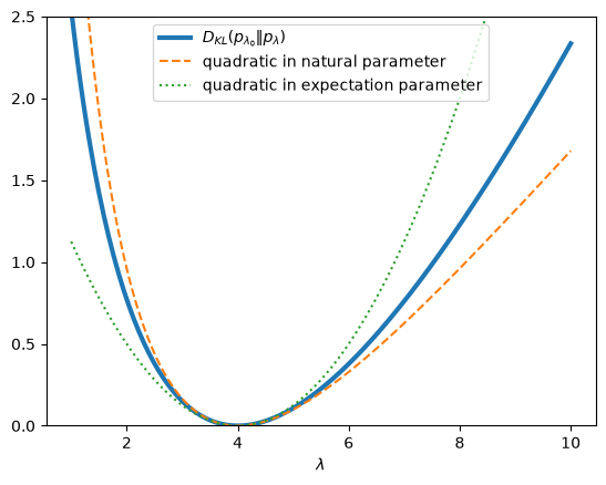
Fig. 22.5 Poisson KL divergence and quadratic approximations#
Near \(\lambda_0\) the three curves coincide; farther away they separate.
22.7. Estimation#
22.7.1. Maximum likelihood matches moments#
Let \(x_1, \ldots, x_n\) be IID draws from a member of the exponential family.
The average log likelihood is
The statistic \(t\) is sufficient: apart from the last term, which does not involve \(\theta\), the likelihood depends on the data only through \(\bar t\).
The average log likelihood is a concave function of \(\theta\) whose first-order condition is \(\nabla F(\hat \theta) = \bar t\).
The maximum likelihood estimator of the expectation parameter is the sample average of the sufficient statistic, \(\hat \eta = \bar t\).
The maximum likelihood estimator of the natural parameter is \(\hat \theta = \nabla F^*(\bar t)\), provided that \(\bar t\) lies in the range of \(\nabla F\).
When it does not, as in a Bernoulli sample with no successes, \(\hat \theta\) does not exist (see Exercise 22.3).
The maximized average log likelihood is \(F^*(\bar t)\) plus the average of \(\log h(x_i)\), by (22.9).
In expectation parameters, maximum likelihood estimation is trivial; in natural parameters, it requires inverting \(\nabla F\).
For the gamma and Beta families, inverting \(\nabla F\) takes a numerical method, such as the Newton iterations we used above.
22.7.2. Finite-sample behavior of the two estimators#
The maximum likelihood estimators in the two coordinate systems behave differently in finite samples.
The estimator \(\hat \eta = \bar t\) is unbiased because it is a sample average; its covariance matrix is \(\operatorname{Cov}_\theta[t(X)]/n = \nabla^2 F(\theta)/n\).
The Fisher information matrix for \(\eta\) is \(\nabla^2 F^*(\eta)\), so the Cramér–Rao lower bound for an unbiased estimator of \(\eta\) is \(\left[\nabla^2 F^*(\eta)\right]^{-1}/n = \nabla^2 F(\theta)/n\).
In expectation parameters, the maximum likelihood estimator is unbiased and attains the Cramér–Rao bound exactly, in every sample size.
The estimator \(\hat \theta = \nabla F^*(\bar t)\) of the natural parameter is a nonlinear function of \(\bar t\), and it is biased in finite samples; for the normal family, \(E \hat \theta = n \theta / (n - 3)\) when \(n > 3\).
The Cramér–Rao bound applies only to unbiased estimators, so for the biased \(\hat \theta\) we treat \(I(\theta)^{-1}/n\) as a benchmark.
In the exponential family, an unbiased estimator can attain the Cramér–Rao bound in finite samples only if the quantity it estimates is an affine function of \(\eta\).
The natural parameter \(\theta = \nabla F^*(\eta)\) is an affine function of \(\eta\) only when \(F\) is quadratic, as for a normal family with known variance.
For the normal family with unknown mean and variance, \(\theta_1 = \eta_1 / (\eta_2 - \eta_1^2)\) and \(\theta_2 = -1/(2(\eta_2 - \eta_1^2))\) are not affine in \(\eta\), so no unbiased estimator of either attains the bound.
For the normal family, as \(n \to \infty\), the bias of \(\hat \theta\) vanishes and \(n\) times its covariance matrix converges to \(I(\theta)^{-1}\).
In general, asymptotic theory describes the distribution of \(\hat \theta\), whose finite-sample moments need not exist, as Exercise 22.3 shows.
The simulation below illustrates these facts for the normal family with \(\mu = 1\) and \(\sigma = 1.5\), using samples of size \(n = 30\).
The ellipses enclose 95 percent of the probability of normal distributions centered at the true parameters, with covariance matrix \(\nabla^2 F(\theta)/n = I(\theta)/n\) in the left panel and \(I(\theta)^{-1}/n\) in the right panel.
def ellipse(center, cov, level=chi2.ppf(0.95, 2), n_points=200):
    """Points on the ellipse (z - center)' cov^{-1} (z - center) = level."""
    angles = np.linspace(0, 2 * np.pi, n_points)
    circle = np.vstack([np.cos(angles), np.sin(angles)])
    return center[:, None] + np.linalg.cholesky(level * cov) @ circle


μ, σ, n, R = 1.0, 1.5, 30, 20_000
θ_true = normal_θ(μ, σ)
η_true = np.array([μ, μ**2 + σ**2])
I_θ = hessian(F_normal, θ_true)        # Fisher information for θ

samples = rng.normal(μ, σ, size=(R, n))
η_hat = np.column_stack([samples.mean(axis=1), (samples**2).mean(axis=1)])
σ2_hat = η_hat[:, 1] - η_hat[:, 0]**2
θ_hat = np.column_stack([η_hat[:, 0] / σ2_hat, -1 / (2 * σ2_hat)])

print("expectation parameters")
print("  bias:", np.round(η_hat.mean(axis=0) - η_true, 4))
print("  n × sample covariance:\n", np.round(n * np.cov(η_hat.T), 3))
print("  n × Cramér–Rao bound = ∇²F(θ):\n", np.round(I_θ, 3))
print("natural parameters")
print("  bias:", np.round(θ_hat.mean(axis=0) - θ_true, 4))
print("  n × sample covariance:\n", np.round(n * np.cov(θ_hat.T), 3))
print("  n × benchmark = I(θ)^{-1}:\n", np.round(np.linalg.inv(I_θ), 3))
print(f"  E θ̂ = nθ/(n-3):", np.round(n * θ_true / (n - 3), 4),
      "  mean of θ̂:", np.round(θ_hat.mean(axis=0), 4))
expectation parameters
  bias: [0.0024 0.0089]
  n × sample covariance:
 [[ 2.221  4.403]
 [ 4.403 18.835]]
  n × Cramér–Rao bound = ∇²F(θ):
 [[ 2.25   4.5  ]
 [ 4.5   19.125]]
natural parameters
  bias: [ 0.0496 -0.024 ]
  n × sample covariance:
 [[ 1.179 -0.294]
 [-0.294  0.145]]
  n × benchmark = I(θ)^{-1}:
 [[ 0.84  -0.198]
 [-0.198  0.099]]
  E θ̂ = nθ/(n-3): [ 0.4938 -0.2469]   mean of θ̂: [ 0.4941 -0.2462]
fig, axes = plt.subplots(1, 2, figsize=(10, 4.5))
panels = ((axes[0], η_hat, η_true, I_θ / n,
           (r"$\hat\eta_1$", r"$\hat\eta_2$"), "expectation parameters",
           "Cramér–Rao ellipse", "lower right"),
          (axes[1], θ_hat, θ_true, np.linalg.inv(I_θ) / n,
           (r"$\hat\theta_1$", r"$\hat\theta_2$"), "natural parameters",
           r"ellipse from $I(\theta)^{-1}/n$", "lower left"))
for ax, est, truth, cov, labels, title, ell_label, loc in panels:
    ax.scatter(*est[:1000].T, s=3, alpha=0.3)
    ax.plot(*ellipse(truth, cov), "k", lw=1.5, label=ell_label)
    ax.plot(*truth, "r+", ms=14, mew=2, label="true value")
    ax.plot(*est.mean(axis=0), "kx", ms=10, mew=2, label="mean of estimates")
    ax.set_xlabel(labels[0])
    ax.set_ylabel(labels[1])
    ax.set_title(title)
    ax.legend(loc=loc)
plt.tight_layout()
plt.show()
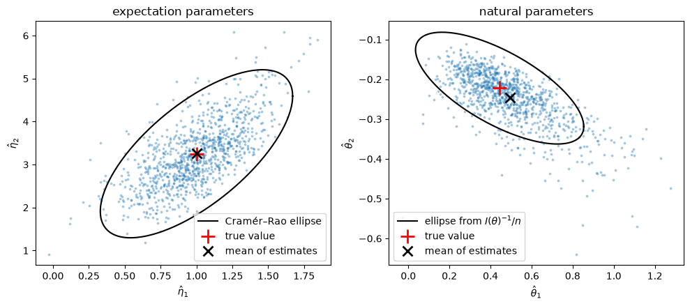
Fig. 22.6 Maximum likelihood estimates in both parameterizations#
In expectation parameters, the cloud of estimates is centered at the true value, and its covariance matrix equals the Cramér–Rao bound, up to simulation error.
In natural parameters, the cloud is skewed, its mean is displaced from the true value by the bias \(3\theta/(n - 3)\), and its covariance matrix is larger than the benchmark \(I(\theta)^{-1}/n\), which it approaches only as \(n\) grows.
22.8. Concluding remarks#
For the exponential family, one convex function \(F\) delivers four facts:
its gradient maps natural parameters \(\theta\) to expectation parameters \(\eta\), and the gradient of its conjugate \(F^*\) maps them back;
its Hessian is the covariance matrix of the sufficient statistic and the Fisher information matrix;
its conjugate is the negative of entropy, when the base measure is constant; and
the Bregman divergences of \(F\) and \(F^*\) are KL divergences.
Members of the exponential family solve maximum entropy problems.
The normal density maximizes entropy among densities with a given mean and variance.
The Lagrange multipliers of a maximum entropy problem are natural parameters and shadow prices.
The logit model’s inclusive value is a log-partition function, and its conjugate is negative entropy.
The sequel Information Projections uses these facts to describe the geometry of KL divergence.
22.9. Exercises#
Exercise 22.1
Consider densities on \((0, \infty)\).
Show that the density that maximizes entropy subject to given values of \(E[X]\) and \(E[\log X]\) is a gamma density, and write the gamma family in the form (22.5).
Compute the log-partition function \(F\), and use (22.6) to express \(E[X]\) and \(E[\log X]\) in terms of the shape and rate parameters.
Draw 500 observations from a gamma distribution with shape \(2.5\) and rate \(1.5\), and compute the maximum likelihood estimator by matching the sample means of \(X\) and \(\log X\), using Newton’s method with the Hessian (22.7). Compare your estimates with those of
scipy.stats.gamma.fitwith the location fixed at zero.
Solution
Here is one solution.
For part 1, the argument that led to (22.2) gives a density proportional to \(\exp(\theta_1 x + \theta_2 \log x) = x^{\theta_2} e^{\theta_1 x}\), which is integrable on \((0, \infty)\) when \(\theta_1 < 0\) and \(\theta_2 > -1\).
This is the gamma density with shape \(a = \theta_2 + 1\) and rate \(b = -\theta_1\):
So \(t(x) = (x, \log x)\), \(\theta = (-b, a - 1)\), and \(h(x) = 1\).
For part 2,
Differentiating,
where \(\psi\) is the digamma function.
The Hessian is
For part 3, we apply Newton’s method to \(\nabla F(\theta) = \bar t\).
We start from the method-of-moments estimates, and we shorten any Newton step that would leave \(\Theta\), where \(a > 0\) and \(b > 0\).
def gamma_mle(x, tol=1e-10, max_iter=100):
    """Match the sample means of x and log x by Newton's method in θ."""
    t_bar = np.array([x.mean(), np.log(x).mean()])
    a = x.mean()**2 / x.var()          # method-of-moments starting values
    b = a / x.mean()
    for _ in range(max_iter):
        grad_F = np.array([a / b, digamma(a) - np.log(b)])
        hess_F = np.array([[a / b**2, 1 / b],
                           [1 / b, polygamma(1, a)]])
        step = np.linalg.solve(hess_F, t_bar - grad_F)  # step in (-b, a - 1)
        s = 1.0
        while b - s * step[0] <= 0 or a + s * step[1] <= 0:
            s /= 2                                      # stay inside Θ
        b, a = b - s * step[0], a + s * step[1]
        if max(abs(s * step[0]) / b, abs(s * step[1]) / a) < tol:
            break
    else:
        raise RuntimeError("no convergence")
    return a, b


rng_gamma = np.random.default_rng(6)
x = rng_gamma.gamma(shape=2.5, scale=1 / 1.5, size=500)
a_hat, b_hat = gamma_mle(x)
a_sp, _, scale_sp = gamma_dist.fit(x, floc=0)
print(f"moment matching: shape = {a_hat:.5f}, rate = {b_hat:.5f}")
print(f"scipy fit:       shape = {a_sp:.5f}, rate = {1 / scale_sp:.5f}")
moment matching: shape = 2.46710, rate = 1.53324
scipy fit:       shape = 2.46710, rate = 1.53324
The two sets of estimates agree.
Exercise 22.2
The Poisson family has the nonconstant base measure \(h(x) = 1/x!\).
Use (22.8) to show that \(F^*(\eta) = \eta \log \eta - \eta\), and check that \(\nabla F^*\) is the inverse of \(\nabla F\).
Show that the entropy of the Poisson(\(\lambda\)) distribution is \(H = \lambda - \lambda \log \lambda + E[\log X!]\), so that \(H = -F^*(\lambda) - E \log h(X)\) and \(F^* \neq -H\). Check the formula numerically for \(\lambda \in \{0.5, 3, 20\}\) by computing \(-\sum_x p(x) \log p(x)\) directly.
Use (22.15) to derive a closed form for \(D_{KL}(\text{Poisson}(\lambda_1) \| \text{Poisson}(\lambda_2))\), and check it against a direct summation.
Solution
Here is one solution.
For part 1, \(F(\theta) = e^\theta\), so the first-order condition for \(\sup_\theta \{\theta \eta - e^\theta\}\) is \(\eta = e^\theta\), or \(\theta = \log \eta\).
Substituting, \(F^*(\eta) = \eta \log \eta - \eta\).
Then \(\nabla F^*(\eta) = \log \eta\), which inverts \(\nabla F(\theta) = e^\theta\).
For part 2, \(\log p(x) = \theta x - e^\theta - \log x!\) with \(\theta = \log \lambda\), so
Because \(E[\log X!] > 0\) whenever \(\lambda > 0\), \(-F^*(\lambda)\) falls short of \(H\), as the last column of the table below shows.
k = np.arange(300)
print(f"{'λ':>5} {'direct H':>10} {'formula':>10} {'-F*(λ)':>10}")
for λ in (0.5, 3.0, 20.0):
    p = poisson.pmf(k, λ)
    H_direct = -p @ poisson.logpmf(k, λ)
    H_formula = λ - λ * np.log(λ) + p @ gammaln(k + 1)
    print(f"{λ:5.1f} {H_direct:10.6f} {H_formula:10.6f} "
          f"{-F_star_poisson(λ):10.6f}")
    λ   direct H    formula     -F*(λ)
  0.5   0.927637   0.927637   0.846574
  3.0   1.931470   1.931470  -0.295837
 20.0   2.912526   2.912526 -39.914645
For part 3, (22.15) gives
which is the formula we used to draw Fig. 22.5.
λ1, λ2 = 3.0, 5.0
direct = poisson.pmf(k, λ1) @ (poisson.logpmf(k, λ1) - poisson.logpmf(k, λ2))
print(f"direct sum:  {direct:.8f}")
print(f"closed form: {λ1 * np.log(λ1 / λ2) - λ1 + λ2:.8f}")
direct sum:  0.46752313
closed form: 0.46752313
Exercise 22.3
Repeat the comparison of the two coordinate systems for the Bernoulli family.
With \(\pi = 0.2\) and \(n = 25\), simulate many samples and compute \(\hat \eta = \bar x\) and \(\hat \theta = \log(\hat \eta / (1 - \hat \eta))\).
Verify that \(\hat \eta\) is unbiased with variance equal to the Cramér–Rao bound \(\pi(1 - \pi)/n\).
What fraction of samples produce an infinite \(\hat \theta\)? Among samples with finite \(\hat \theta\), compare the mean and variance of \(\hat \theta\) with \(\theta\) and with the benchmark \(1/(n \pi (1 - \pi))\). How do these comparisons change when \(n = 400\)?
Solution
Here is one solution.
def bernoulli_experiment(π, n, rng, R=100_000):
    η_hat = rng.binomial(n, π, size=R) / n
    θ = np.log(π / (1 - π))
    finite = (η_hat > 0) & (η_hat < 1)
    θ_hat = np.log(η_hat[finite] / (1 - η_hat[finite]))
    print(f"n = {n}")
    print(f"  η̂: mean {η_hat.mean():.4f} (π = {π}), "
          f"variance {η_hat.var():.6f} (bound {π * (1 - π) / n:.6f})")
    print(f"  fraction with infinite θ̂: {1 - finite.mean():.4f}")
    print(f"  finite θ̂: mean {θ_hat.mean():.4f} (θ = {θ:.4f}), "
          f"variance {θ_hat.var():.4f} "
          f"(benchmark {1 / (n * π * (1 - π)):.4f})")


rng_bern = np.random.default_rng(2)
bernoulli_experiment(0.2, 25, rng_bern)
bernoulli_experiment(0.2, 400, rng_bern)
n = 25
  η̂: mean 0.2002 (π = 0.2), variance 0.006404 (bound 0.006400)
  fraction with infinite θ̂: 0.0037
  finite θ̂: mean -1.4672 (θ = -1.3863), variance 0.3075 (benchmark 0.2500)
n = 400
  η̂: mean 0.2000 (π = 0.2), variance 0.000399 (bound 0.000400)
  fraction with infinite θ̂: 0.0000
  finite θ̂: mean -1.3907 (θ = -1.3863), variance 0.0158 (benchmark 0.0156)
With \(n = 25\), about \(0.4\) percent of samples contain no successes.
In those samples \(\bar x = 0\) lies on the boundary of the range of \(\nabla F\), the interval \((0, 1)\), so the maximum likelihood estimator of \(\theta\) does not exist; the formula gives \(\hat \theta = -\infty\).
Among the other samples, \(\hat \theta\) is biased downward, with a variance more than 20 percent above the benchmark \(1/(n \pi (1 - \pi))\).
With \(n = 400\), infinite estimates essentially never occur, and the bias and the gap between the variance and the benchmark are small, as asymptotic theory predicts.
Meanwhile \(\hat \eta\) is unbiased and attains the Cramér–Rao bound at both sample sizes.
Exercise 22.4
Bayes’ law takes a simple form in natural parameters.
Let \(x_1, \ldots, x_n\) be IID Bernoulli(\(\pi\)) draws, and let the prior for \(\pi\) be Beta(\(a\), \(b\)). Using the Beta row of the table above, write the prior as a member of the Beta family with natural parameters \((a - 1, b - 1)\) and show that the posterior is a member of the same family whose natural parameters are those of the prior plus \(\left(\sum_i x_i, \, n - \sum_i x_i\right)\).
Explain why, more generally, if the log likelihood is linear in some functions of the parameter and the prior is a member of the exponential family with those functions as its sufficient statistic, the posterior is in the same family and Bayes’ law adds to its natural parameters.
Starting from a Beta(1, 1) prior and draws with \(\pi = 0.3\), plot the posterior mean of \(\pi\), with a band of two posterior standard deviations, as a function of \(n\). After \(n = 200\) draws, use (22.6) and (22.7) to compute the posterior mean and variance of \(\log \pi\), and check them by Monte Carlo.
The Beta–Bernoulli model appears in Exchangeability and Bayesian Updating, Likelihood Ratio Processes and Bayesian Learning, and Merging of Opinions: The Blackwell–Dubins Theorem.
Solution
Here is one solution.
For part 1, the prior density is proportional to \(\pi^{a - 1}(1 - \pi)^{b - 1} = \exp\left( (a - 1) \log \pi + (b - 1) \log(1 - \pi) \right)\).
The likelihood of \(n\) draws with \(s = \sum_i x_i\) successes is \(\pi^s (1 - \pi)^{n - s} = \exp\left( s \log \pi + (n - s) \log (1 - \pi) \right)\).
Multiplying, the posterior is proportional to \(\exp\left( (a - 1 + s) \log \pi + (b - 1 + n - s) \log(1 - \pi) \right)\), a Beta(\(a + s\), \(b + n - s\)) density.
Its natural parameters are \((a - 1 + s, b - 1 + n - s)\).
For part 2, Bayes’ law says that the log posterior equals the log prior plus the log likelihood, up to a constant.
If the log likelihood is linear in some functions of the parameter, as it is in \((\log \pi, \log(1 - \pi))\) here, and the log prior is linear in the same functions, then the log posterior is too, with coefficients that add.
The prior family whose sufficient statistics are those functions of the parameter is called a conjugate family.
This use of the word conjugate is unrelated to the convex conjugate \(F^*\).
For part 3, the posterior mean of \(\pi\) is \((a + s)/(a + b + n)\), and the posterior variance is \((a + s)(b + n - s) / \left((a + b + n)^2 (a + b + n + 1)\right)\).
rng_bayes = np.random.default_rng(3)
π_true, a0, b0 = 0.3, 1.0, 1.0
x = rng_bayes.binomial(1, π_true, size=500)
s = np.cumsum(x)
n_vals = np.arange(1, x.size + 1)
a_post, b_post = a0 + s, b0 + n_vals - s

post_mean = a_post / (a_post + b_post)
post_sd = np.sqrt(a_post * b_post
                  / ((a_post + b_post)**2 * (a_post + b_post + 1)))
fig, ax = plt.subplots()
ax.plot(n_vals, post_mean, label="posterior mean")
ax.fill_between(n_vals, post_mean - 2 * post_sd, post_mean + 2 * post_sd,
                alpha=0.3, label="± 2 posterior standard deviations")
ax.axhline(π_true, color="k", ls="--", lw=1, label=r"true $\pi$")
ax.set_xlabel("$n$")
ax.set_ylim(0, 1)
ax.legend()
plt.show()
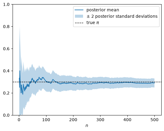
After \(n = 200\) draws the posterior is Beta(\(a\), \(b\)) with \((a, b) = (a_0 + s, b_0 + 200 - s)\).
Applying (22.6) to \(F(\theta) = \log B(\theta_1 + 1, \theta_2 + 1)\) gives \(E[\log \pi] = \psi(a) - \psi(a + b)\), and (22.7) gives \(\operatorname{Var}[\log \pi] = \psi'(a) - \psi'(a + b)\).
a, b = a_post[199], b_post[199]
draws = rng_bayes.beta(a, b, size=200_000)
print(f"E[log π]:   formula {digamma(a) - digamma(a + b):.5f}, "
      f"Monte Carlo {np.log(draws).mean():.5f}")
print(f"Var[log π]: formula {polygamma(1, a) - polygamma(1, a + b):.5f}, "
      f"Monte Carlo {np.log(draws).var():.5f}")
E[log π]:   formula -1.27154, Monte Carlo -1.27141
Var[log π]: formula 0.01274, Monte Carlo 0.01273