24. Likelihood Processes for VAR Models

Contents

• Likelihood Processes for VAR Models

  • Overview

  • VAR model setup

  • Likelihood ratio process

  • Example 1: Two AR(1) processes

  • Example 2: Bivariate VAR models

  • Application: Samuelson multiplier-accelerator

24.1. Overview

This lecture extends our analysis of likelihood ratio processes to Vector Autoregressions (VARs).

We’ll

• Construct likelihood functions for VAR models

• Form likelihood ratio processes for comparing two VAR models

• Visualize the evolution of likelihood ratios over time

• Connect VAR likelihood ratios to the Samuelson multiplier-accelerator model

Our analysis builds on concepts from:

• Likelihood Ratio Processes

• Linear State Space Models

• Samuelson Multiplier-Accelerator

Let’s start by importing helpful libraries:

import numpy as np
import matplotlib.pyplot as plt
from scipy import linalg
from scipy.stats import multivariate_normal as mvn
from quantecon import LinearStateSpace
import quantecon as qe
from numba import jit
from typing import NamedTuple, Optional, Tuple
from collections import namedtuple

24.2. VAR model setup

Consider a VAR model of the form:

\[\begin{split} \begin{aligned} x_{t+1} & = A x_t + C w_{t+1} \\ x_0 & \sim \mathcal{N}(\mu_0, \Sigma_0) \end{aligned} \end{split}\]

where:

• \(x_t\) is an \(n \times 1\) state vector

• \(w_{t+1} \sim \mathcal{N}(0, I)\) is an \(m \times 1\) vector of shocks

• \(A\) is an \(n \times n\) transition matrix

• \(C\) is an \(n \times m\) volatility matrix

Let’s define the necessary data structures for the VAR model

VARModel = namedtuple('VARModel', ['A', 'C', 'μ_0', 'Σ_0',        
                                    'CC', 'CC_inv', 'log_det_CC', 
                                    'Σ_0_inv', 'log_det_Σ_0'])
def compute_stationary_var(A, C):
    """
    Compute stationary mean and covariance for VAR model
    """
    n = A.shape[0]
    
    # Check stability
    eigenvalues = np.linalg.eigvals(A)
    if np.max(np.abs(eigenvalues)) >= 1:
        raise ValueError("VAR is not stationary")
    
    μ_0 = np.zeros(n)
    
    # Stationary covariance: solve discrete Lyapunov equation
    # Σ_0 = A @ Σ_0 @ A.T + C @ C.T
    CC = C @ C.T
    Σ_0 = linalg.solve_discrete_lyapunov(A, CC)
    
    return μ_0, Σ_0

def create_var_model(A, C, μ_0=None, Σ_0=None, stationary=True):
    """
    Create a VAR model with parameters and precomputed matrices
    """
    A = np.asarray(A)
    C = np.asarray(C)
    n = A.shape[0]
    CC = C @ C.T
    
    if stationary:
        μ_0_comp, Σ_0_comp = compute_stationary_var(A, C)
    else:
        μ_0_comp = μ_0 if μ_0 is not None else np.zeros(n)
        Σ_0_comp = Σ_0 if Σ_0 is not None else np.eye(n)
    
    # Check if CC is singular
    det_CC = np.linalg.det(CC)
    if np.abs(det_CC) < 1e-10:
        # Use pseudo-inverse for singular case
        CC_inv = np.linalg.pinv(CC)
        CC_reg = CC + 1e-10 * np.eye(CC.shape[0])
        log_det_CC = np.log(np.linalg.det(CC_reg))
    else:
        CC_inv = np.linalg.inv(CC)
        log_det_CC = np.log(det_CC)
    
    # Same check for Σ_0
    det_Σ_0 = np.linalg.det(Σ_0_comp)
    if np.abs(det_Σ_0) < 1e-10:
        Σ_0_inv = np.linalg.pinv(Σ_0_comp)
        Σ_0_reg = Σ_0_comp + 1e-10 * np.eye(Σ_0_comp.shape[0])
        log_det_Σ_0 = np.log(np.linalg.det(Σ_0_reg))
    else:
        Σ_0_inv = np.linalg.inv(Σ_0_comp)
        log_det_Σ_0 = np.log(det_Σ_0)
    
    return VARModel(A=A, C=C, μ_0=μ_0_comp, Σ_0=Σ_0_comp,
                    CC=CC, CC_inv=CC_inv, log_det_CC=log_det_CC,
                    Σ_0_inv=Σ_0_inv, log_det_Σ_0=log_det_Σ_0)

24.2.1. Joint distribution

The joint probability distribution \(f(x_T, x_{T-1}, \ldots, x_0)\) can be factored as:

\[ f(x_T, \ldots, x_0) = f(x_T | x_{T-1}) f(x_{T-1} | x_{T-2}) \cdots f(x_1 | x_0) f(x_0) \]

Since the VAR is Markovian, \(f(x_{t+1} | x_t, \ldots, x_0) = f(x_{t+1} | x_t)\).

24.2.2. Conditional densities

Given the Gaussian structure, the conditional distribution \(f(x_{t+1} | x_t)\) is Gaussian with:

• Mean: \(A x_t\)

• Covariance: \(CC'\)

The log conditional density is:

\[ \log f(x_{t+1} | x_t) = -\frac{n}{2} \log(2\pi) - \frac{1}{2} \log \det(CC') - \frac{1}{2} (x_{t+1} - A x_t)' (CC')^{-1} (x_{t+1} - A x_t) \]

def log_likelihood_transition(x_next, x_curr, model):
    """
    Compute log likelihood of transition from x_curr to x_next
    """
    x_next = np.atleast_1d(x_next)
    x_curr = np.atleast_1d(x_curr)
    n = len(x_next)
    diff = x_next - model.A @ x_curr
    return -0.5 * (n * np.log(2 * np.pi) + model.log_det_CC + 
                  diff @ model.CC_inv @ diff)

The log density of the initial state is:

\[ \log f(x_0) = -\frac{n}{2} \log(2\pi) - \frac{1}{2} \log \det(\Sigma_0) - \frac{1}{2} (x_0 - \mu_0)' \Sigma_0^{-1} (x_0 - \mu_0) \]

def log_likelihood_initial(x_0, model):
    """
    Compute log likelihood of initial state
    """
    x_0 = np.atleast_1d(x_0)
    n = len(x_0)
    diff = x_0 - model.μ_0
    return -0.5 * (n * np.log(2 * np.pi) + model.log_det_Σ_0 + 
                  diff @ model.Σ_0_inv @ diff)

Now let’s group the likelihood computations into a single function that computes the log likelihood of an entire path

def log_likelihood_path(X, model):
    """
    Compute log likelihood of entire path
    """

    T = X.shape[0] - 1
    log_L = log_likelihood_initial(X[0], model)
    
    for t in range(T):
        log_L += log_likelihood_transition(X[t+1], X[t], model)
        
    return log_L

def simulate_var(model, T, N_paths=1):
    """
    Simulate paths from the VAR model
    """
    n = model.A.shape[0]
    m = model.C.shape[1]
    paths = np.zeros((N_paths, T+1, n))
    
    for i in range(N_paths):
        # Draw initial state
        x = mvn.rvs(mean=model.μ_0, cov=model.Σ_0)
        x = np.atleast_1d(x)
        paths[i, 0] = x
        
        # Simulate forward
        for t in range(T):
            w = np.random.randn(m)
            x = model.A @ x + model.C @ w
            paths[i, t+1] = x
            
    return paths if N_paths > 1 else paths[0]

24.3. Likelihood ratio process

Now let’s compute likelihood ratio processes for comparing two VAR models

def compute_likelihood_ratio_var(paths, model_f, model_g):
    """
    Compute likelihood ratio process for VAR models
    """
    if paths.ndim == 2:
        paths = paths[np.newaxis, :]
    
    N_paths, T_plus_1, n = paths.shape
    T = T_plus_1 - 1
    log_L_ratios = np.zeros((N_paths, T+1))
    
    for i in range(N_paths):
        X = paths[i]
        
        # Initial log likelihood ratio
        log_L_f_0 = log_likelihood_initial(X[0], model_f)
        log_L_g_0 = log_likelihood_initial(X[0], model_g)
        log_L_ratios[i, 0] = log_L_f_0 - log_L_g_0
        
        # Recursive computation
        for t in range(1, T+1):
            log_L_f_t = log_likelihood_transition(X[t], X[t-1], model_f)
            log_L_g_t = log_likelihood_transition(X[t], X[t-1], model_g)
            
            # Update log likelihood ratio
            log_diff = log_L_f_t - log_L_g_t
            
            log_L_prev = log_L_ratios[i, t-1]
            log_L_new = log_L_prev + log_diff
            log_L_ratios[i, t] = log_L_new

    return log_L_ratios if N_paths > 1 else log_L_ratios[0]

24.4. Example 1: Two AR(1) processes

Let’s start with a simple example comparing two univariate AR(1) processes with \(A_f = 0.8\), \(A_g = 0.5\), and \(C_f = 0.3\), \(C_g = 0.4\)

# Model f: AR(1) with persistence ρ = 0.8
A_f = np.array([[0.8]])
C_f = np.array([[0.3]])

# Model g: AR(1) with persistence ρ = 0.5
A_g = np.array([[0.5]])
C_g = np.array([[0.4]])

# Create VAR models
model_f = create_var_model(A_f, C_f)
model_g = create_var_model(A_g, C_g)

Let’s generate 100 paths of length 200 from model \(f\) and compute the likelihood ratio processes

# Simulate from model f
T = 200
N_paths = 100
paths_from_f = simulate_var(model_f, T, N_paths)

L_ratios_f = compute_likelihood_ratio_var(paths_from_f, model_f, model_g)

fig, ax = plt.subplots()

for i in range(min(20, N_paths)):
    ax.plot(L_ratios_f[i], alpha=0.3, color='C0', lw=2)

ax.axhline(y=0, color='gray', linestyle='--', alpha=0.5)
ax.set_ylabel(r'$\log L_t$')
ax.set_title('log likelihood ratio processes (nature = f)')

plt.tight_layout()
plt.show()

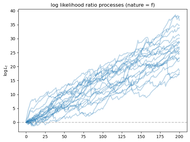
As we expected, the likelihood ratio processes goes to \(+\infty\) as \(T\) increases, indicating that model \(f\) is chosen correctly by our algorithm.

24.5. Example 2: Bivariate VAR models

Now let’s consider an example with bivariate VAR models with

\[\begin{split} A_f & = \begin{bmatrix} 0.7 & 0.2 \\ 0.1 & 0.6 \end{bmatrix}, \quad C_f = \begin{bmatrix} 0.3 & 0.1 \\ 0.1 & 0.3 \end{bmatrix} \end{split}\]

and

\[\begin{split} A_g & = \begin{bmatrix} 0.5 & 0.3 \\ 0.2 & 0.5 \end{bmatrix}, \quad C_g = \begin{bmatrix} 0.4 & 0.0 \\ 0.0 & 0.4 \end{bmatrix} \end{split}\]

A_f = np.array([[0.7, 0.2],
                 [0.1, 0.6]])

C_f = np.array([[0.3, 0.1],
                 [0.1, 0.3]])

A_g = np.array([[0.5, 0.3],
                 [0.2, 0.5]])

C_g = np.array([[0.4, 0.0],
                 [0.0, 0.4]])

# Create VAR models
model2_f = create_var_model(A_f, C_f)
model2_g = create_var_model(A_g, C_g)

# Check stationarity
print("model f eigenvalues:", np.linalg.eigvals(A_f))
print("model g eigenvalues:", np.linalg.eigvals(A_g))

model f eigenvalues: [0.8 0.5]
model g eigenvalues: [0.74494897 0.25505103]

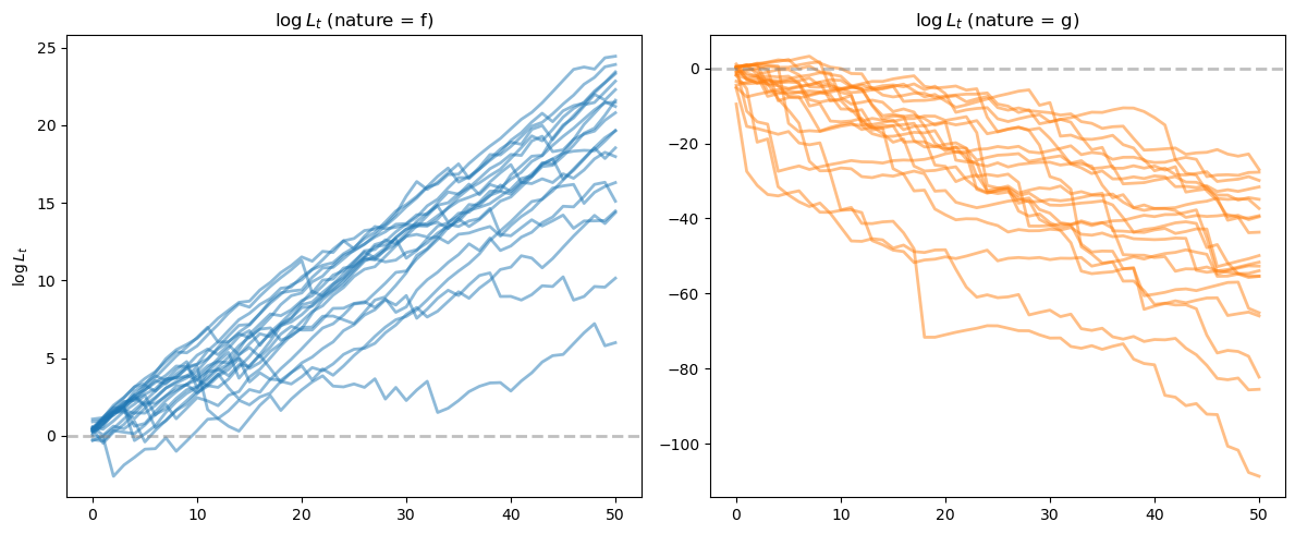
Let’s generate 50 paths of length 50 from both models and compute the likelihood ratio processes

# Simulate from both models
T = 50
N_paths = 50

paths_from_f = simulate_var(model2_f, T, N_paths)
paths_from_g = simulate_var(model2_g, T, N_paths)

# Compute likelihood ratios
L_ratios_ff = compute_likelihood_ratio_var(paths_from_f, model2_f, model2_g)
L_ratios_gf = compute_likelihood_ratio_var(paths_from_g, model2_f, model2_g)

We can see that for paths generated from model \(f\), the likelihood ratio processes tend to go to \(+\infty\), while for paths from model \(g\), they tend to go to \(-\infty\).

# Visualize the results
fig, axes = plt.subplots(1, 2, figsize=(12, 5))

ax = axes[0]
for i in range(min(20, N_paths)):
    ax.plot(L_ratios_ff[i], alpha=0.5, color='C0', lw=2)
ax.axhline(y=0, color='gray', linestyle='--', alpha=0.5, lw=2)
ax.set_title(r'$\log L_t$ (nature = f)')
ax.set_ylabel(r'$\log L_t$')

ax = axes[1]
for i in range(min(20, N_paths)):
    ax.plot(L_ratios_gf[i], alpha=0.5, color='C1', lw=2)
ax.axhline(y=0, color='gray', linestyle='--', alpha=0.5, lw=2)
ax.set_title(r'$\log L_t$ (nature = g)')
plt.tight_layout()
plt.show()

Let’s apply a Neyman-Pearson frequentist decision rule described in Likelihood Ratio Processes that selects model \(f\) when \(\log L_T \geq 0\) and model \(g\) when \(\log L_T < 0\)

fig, ax = plt.subplots()
T_values = np.arange(0, T+1)
accuracy_f = np.zeros(len(T_values))
accuracy_g = np.zeros(len(T_values))

for i, t in enumerate(T_values):
    # Correct selection when data from f
    accuracy_f[i] = np.mean(L_ratios_ff[:, t] > 0)
    # Correct selection when data from g
    accuracy_g[i] = np.mean(L_ratios_gf[:, t] < 0)

ax.plot(T_values, accuracy_f, 'C0', linewidth=2, label='accuracy (nature = f)')
ax.plot(T_values, accuracy_g, 'C1', linewidth=2, label='accuracy (nature = g)')
ax.axhline(y=0.5, color='gray', linestyle='--', alpha=0.5)
ax.set_xlabel('T')
ax.set_ylabel('accuracy')
ax.legend()

plt.tight_layout()
plt.show()

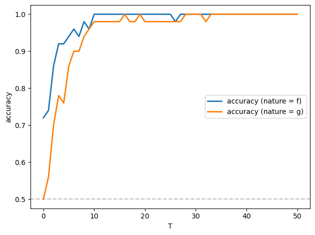
Evidently, the accuracy approaches \(1\) as \(T\) increases, and it does so very quickly.

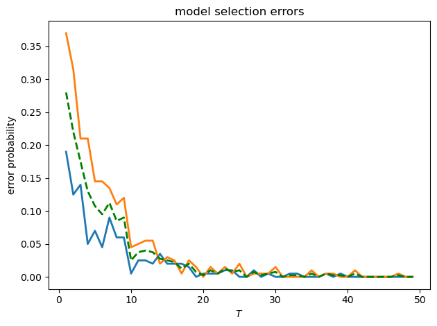
Let’s also check the type I and type II errors as functions of \(T\)

def model_selection_analysis(T_values, model_f, model_g, N_sim=500):
    """
    Analyze model selection performance for different sample sizes
    """
    errors_f = []  # Type I errors
    errors_g = []  # Type II errors
    
    for T in T_values:
        # Simulate from model f
        paths_f = simulate_var(model_f, T, N_sim//2)
        L_ratios_f = compute_likelihood_ratio_var(paths_f, model_f, model_g)
        
        # Simulate from model g
        paths_g = simulate_var(model_g, T, N_sim//2)
        L_ratios_g = compute_likelihood_ratio_var(paths_g, model_f, model_g)
        
        # Decision rule: choose f if log L_T >= 0
        errors_f.append(np.mean(L_ratios_f[:, -1] < 0))
        errors_g.append(np.mean(L_ratios_g[:, -1] >= 0))
    
    return np.array(errors_f), np.array(errors_g)

T_values = np.arange(1, 50, 1)
errors_f, errors_g = model_selection_analysis(T_values, model2_f, model2_g, N_sim=400)

fig, ax = plt.subplots()

ax.plot(T_values, errors_f, 'C0', linewidth=2, label='type I error')
ax.plot(T_values, errors_g, 'C1', linewidth=2, label='type II error')
ax.plot(T_values, 0.5 * (errors_f + errors_g), 'g--', 
linewidth=2, label='average error')
ax.set_xlabel('$T$')
ax.set_ylabel('error probability')
ax.set_title('model selection errors')
plt.tight_layout()
plt.show()

24.6. Application: Samuelson multiplier-accelerator

Now let’s connect to the Samuelson multiplier-accelerator model.

The model consists of:

• Consumption: \(C_t = \gamma + a Y_{t-1}\) where \(a \in (0,1)\) is the marginal propensity to consume

• Investment: \(I_t = b(Y_{t-1} - Y_{t-2})\) where \(b > 0\) is the accelerator coefficient

• Government spending: \(G_t = G\) (constant)

We have the national income identity

\[ Y_t = C_t + I_t + G_t \]

Equations yields the second-order difference equation:

\[ Y_t = (\gamma + G) + (a + b)Y_{t-1} - b Y_{t-2} + \sigma \epsilon_t \]

With \(\rho_1 = a + b\) and \(\rho_2 = -b\), we have:

\[ Y_t = (\gamma + G) + \rho_1 Y_{t-1} + \rho_2 Y_{t-2} + \sigma \epsilon_t \]

To fit into our discussion, we write it into state-space representation.

To handle the constant term properly, we use an augmented state vector \(\mathbf{x}_t = [1, Y_t, Y_{t-1}]'\):

\[\begin{split} \mathbf{x}_{t+1} = \begin{bmatrix} 1 \\ Y_{t+1} \\ Y_t \end{bmatrix} = \begin{bmatrix} 1 & 0 & 0 \\ \gamma + G & \rho_1 & \rho_2 \\ 0 & 1 & 0 \end{bmatrix} \begin{bmatrix} 1 \\ Y_t \\ Y_{t-1} \end{bmatrix} + \begin{bmatrix} 0 \\ \sigma \\ 0 \end{bmatrix} \epsilon_{t+1} \end{split}\]

The observation equation extracts the economic variables:

\[\begin{split} \mathbf{y}_t = \begin{bmatrix} Y_t \\ C_t \\ I_t \end{bmatrix} = \begin{bmatrix} \gamma + G & \rho_1 & \rho_2 \\ \gamma & a & 0 \\ 0 & b & -b \end{bmatrix} \begin{bmatrix} 1 \\ Y_t \\ Y_{t-1} \end{bmatrix} \end{split}\]

This gives us:

• \(Y_t = (\gamma + G) \cdot 1 + \rho_1 Y_{t-1} + \rho_2 Y_{t-2}\) (total output)

• \(C_t = \gamma \cdot 1 + a Y_{t-1}\) (consumption)

• \(I_t = b(Y_{t-1} - Y_{t-2})\) (investment)

def samuelson_to_var(a, b, γ, G, σ):
    """
    Convert Samuelson model parameters to VAR form with augmented state
    
    Samuelson model:
    - Y_t = C_t + I_t + G
    - C_t = γ + a*Y_{t-1}
    - I_t = b*(Y_{t-1} - Y_{t-2})
    
    Reduced form: Y_t = (γ+G) + (a+b)*Y_{t-1} - b*Y_{t-2} + σ*ε_t
    
    State vector is [1, Y_t, Y_{t-1}]'
    """
    ρ_1 = a + b
    ρ_2 = -b
    
    # State transition matrix for augmented state
    A = np.array([[1,      0,     0],
                  [γ + G,  ρ_1,   ρ_2],
                  [0,      1,     0]])
    
    # Shock loading matrix
    C = np.array([[0],
                  [σ],
                  [0]])
    
    # Observation matrix (extracts Y_t, C_t, I_t)
    G_obs = np.array([[γ + G,  ρ_1,  ρ_2],   # Y_t
                      [γ,      a,    0],     # C_t
                      [0,      b,   -b]])    # I_t
    
    return A, C, G_obs

We define functions in the code cell below to get the initial conditions and check stability

Show code cell source

Hide code cell source

def get_samuelson_initial_conditions(a, b, γ, G, y_0=None, y_m1=None, 
                                    stationary_init=False):
    """
    Get initial conditions for Samuelson model
    """
    # Calculate steady state
    y_ss = (γ + G) / (1 - a - b)
    
    if y_0 is None:
        y_0 = y_ss
    if y_m1 is None:
        y_m1 = y_ss if stationary_init else y_0 * 0.95
    
    # Initial mean
    μ_0 = np.array([1.0, y_0, y_m1])
    
    if stationary_init:
        Σ_0 = np.array([[0,  0,    0],
                        [0,  1,    0.5],
                        [0,  0.5,  1]])
    else:
        Σ_0 = np.array([[0,  0,    0],
                        [0,  25,   15],
                        [0,  15,   25]])
    
    return μ_0, Σ_0

def check_samuelson_stability(a, b):
    """
    Check stability of Samuelson model and return characteristic roots
    """
    ρ_1 = a + b
    ρ_2 = -b

    roots = np.roots([1, -ρ_1, -ρ_2])
    max_abs_root = np.max(np.abs(roots))
    is_stable = max_abs_root < 1
    
    # Determine type of dynamics
    if np.iscomplex(roots[0]):
        if max_abs_root < 1:
            dynamics = "Damped oscillations"
        else:
            dynamics = "Explosive oscillations"
    else:
        if max_abs_root < 1:
            dynamics = "Smooth convergence"
        else:
            if np.max(roots) > 1:
                dynamics = "Explosive growth"
            else:
                dynamics = "Explosive oscillations (real roots)"
    
    return is_stable, roots, max_abs_root, dynamics

Let’s implement it and inspect the likelihood ratio processes induced by two Samuelson models with different parameters.

def create_samuelson_var_model(a, b, γ, G, σ, stationary_init=False,
                               y_0=None, y_m1=None):
    """
    Create a VAR model from Samuelson parameters
    """
    A, C, G_obs = samuelson_to_var(a, b, γ, G, σ)
    
    μ_0, Σ_0 = get_samuelson_initial_conditions(
        a, b, γ, G, y_0, y_m1, stationary_init
    )
    
    # Create VAR model
    model = create_var_model(A, C, μ_0, Σ_0, stationary=False)
    is_stable, roots, max_root, dynamics = check_samuelson_stability(a, b)
    info = {
        'a': a, 'b': b, 'γ': γ, 'G': G, 'σ': σ,
        'ρ_1': a + b, 'ρ_2': -b,
        'steady_state': (γ + G) / (1 - a - b),
        'is_stable': is_stable,
        'roots': roots,
        'max_abs_root': max_root,
        'dynamics': dynamics
    }
    
    return model, G_obs, info

def simulate_samuelson(model, G_obs, T, N_paths=1):
    """
    Simulate Samuelson model
    """
    # Simulate state paths
    states = simulate_var(model, T, N_paths)
    
    # Extract observables using G matrix
    if N_paths == 1:
        # Single path: states is (T+1, 3)
        observables = (G_obs @ states.T).T
    else:
        # Multiple paths: states is (N_paths, T+1, 3)
        observables = np.zeros((N_paths, T+1, 3))
        for i in range(N_paths):
            observables[i] = (G_obs @ states[i].T).T
    
    return states, observables

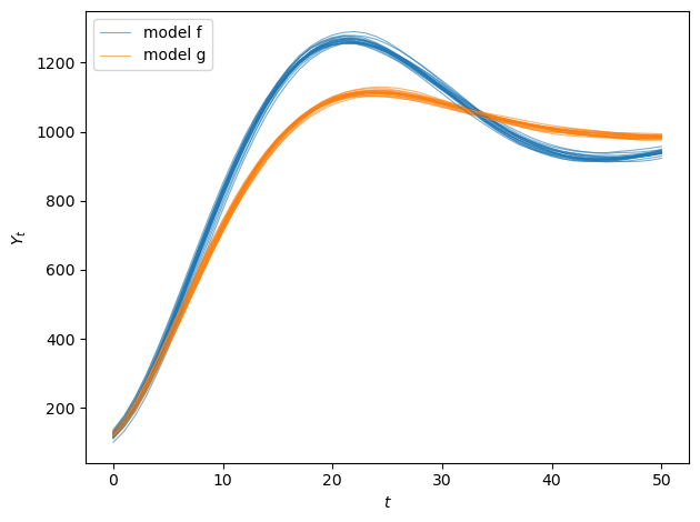
Now let’s simulate two Samuelson models with different accelerator coefficients and plot their sample paths

# Model f: Higher accelerator coefficient
a_f, b_f = 0.98, 0.9
γ_f, G_f, σ_f = 10, 10, 0.5

# Model g: Lower accelerator coefficient  
a_g, b_g = 0.98, 0.85
γ_g, G_g, σ_g = 10, 10, 0.5


model_sam_f, G_obs_f, info_f = create_samuelson_var_model(
    a_f, b_f, γ_f, G_f, σ_f, 
    stationary_init=False, 
    y_0=100, y_m1=95
)

model_sam_g, G_obs_g, info_g = create_samuelson_var_model(
    a_g, b_g, γ_g, G_g, σ_g,
    stationary_init=False,
    y_0=100, y_m1=95
)

T = 50
N_paths = 50

# Get both states and observables
states_f, obs_f = simulate_samuelson(model_sam_f, G_obs_f, T, N_paths)
states_g, obs_g = simulate_samuelson(model_sam_g, G_obs_g, T, N_paths)

output_paths_f = obs_f[:, :, 0] 
output_paths_g = obs_g[:, :, 0]
    
print("model f:")
print(f"  ρ_1 = a + b = {info_f['ρ_1']:.2f}")
print(f"  ρ_2 = -b = {info_f['ρ_2']:.2f}")
print(f"  roots: {info_f['roots']}")
print(f"  dynamics: {info_f['dynamics']}")

print("\nmodel g:")
print(f"  ρ_1 = a + b = {info_g['ρ_1']:.2f}")
print(f"  ρ_2 = -b = {info_g['ρ_2']:.2f}")
print(f"  roots: {info_g['roots']}")
print(f"  dynamics: {info_g['dynamics']}")


fig, ax = plt.subplots(1, 1)

for i in range(min(20, N_paths)):
    ax.plot(output_paths_f[i], alpha=0.6, color='C0', linewidth=0.8)
    ax.plot(output_paths_g[i], alpha=0.6, color='C1', linewidth=0.8)
ax.set_xlabel('$t$')
ax.set_ylabel('$Y_t$')
ax.legend(['model f', 'model g'], loc='upper left')
plt.tight_layout()
plt.show()

model f:
  ρ_1 = a + b = 1.88
  ρ_2 = -b = -0.90
  roots: [0.94+0.12806248j 0.94-0.12806248j]
  dynamics: Damped oscillations

model g:
  ρ_1 = a + b = 1.83
  ρ_2 = -b = -0.85
  roots: [0.915+0.11302655j 0.915-0.11302655j]
  dynamics: Damped oscillations

# Compute likelihood ratios
L_ratios_ff = compute_likelihood_ratio_var(states_f, model_sam_f, model_sam_g)
L_ratios_gf = compute_likelihood_ratio_var(states_g, model_sam_f, model_sam_g) 

fig, axes = plt.subplots(1, 2, figsize=(12, 5))

ax = axes[0]
for i in range(min(20, N_paths)):
    ax.plot(L_ratios_ff[i], alpha=0.5, color='C0', lw=0.8)
ax.axhline(y=0, color='gray', linestyle='--', alpha=0.5)
ax.set_title(r'$\log L_t$ (nature = f)')
ax.set_ylabel(r'$\log L_t$')

ax = axes[1]
for i in range(min(20, N_paths)):
    ax.plot(L_ratios_gf[i], alpha=0.5, color='C1', lw=0.8)
ax.axhline(y=0, color='gray', linestyle='--', alpha=0.5)
ax.set_title(r'$\log L_t$ (nature = g)')
plt.show()

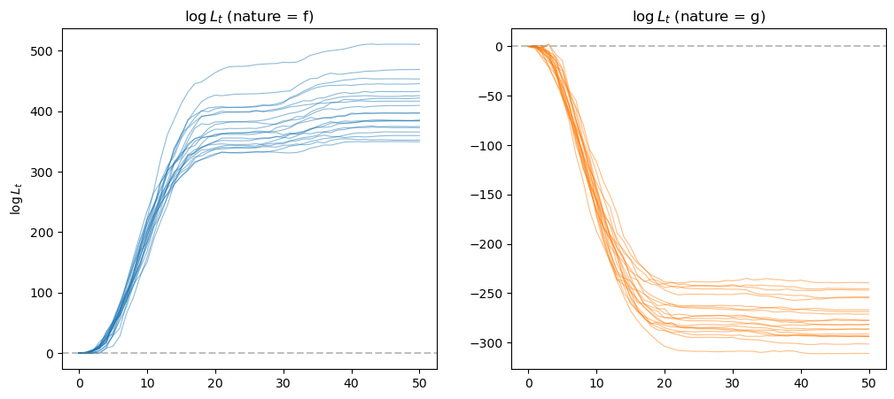
In the figure on the left, data are generated by \(f\) and the likelihood ratio diverges to plus infinity.

In the figure on the right, data are generated by \(g\) and the likelihood ratio diverges to negative infinity.

In both cases, we applied a lower and upper threshold for the log likelihood ratio process for numerical stability since they grow unbounded very quickly.

In both cases, the likelihood ratio processes eventually lead us to select the correct model.