77. Robust Permanent Income and Pricing#
In addition to what’s in Anaconda, this lecture will need the following libraries:
!pip install --upgrade quantecon
77.1. Overview#
This lecture studies the model of [Hansen et al., 1999] — Lars Peter Hansen, Thomas J. Sargent, and Thomas D. Tallarini’s “Robust Permanent Income and Pricing”.
The paper asks a simple question with surprising consequences.
What happens to a classic permanent income consumer when, instead of trusting a single probability model of their income, they fear that their model is misspecified and want decisions that work well across a family of nearby models?
Such a consumer is called a robust decision maker.
The central findings are:
A preference for robustness is hidden inside the quantity implications of the ordinary permanent income model.
Robustness and risk-sensitivity are two interpretations of the same decision rules — a single parameter \(\sigma\) governs both.
Concern about small amounts of model misspecification can show up as large market-based measures of risk aversion.
The consumption and savings data alone cannot identify the robustness parameter: the model is observationally equivalent to a standard permanent income model with a lower discount factor.
But asset prices — in particular the market price of risk — can be used to pin robustness down.
We will learn about
risk-sensitive recursive preferences and the operator \(\mathcal{R}_t\)
how a malevolent “second agent” implements a preference for robustness through a two-player zero-sum game
the link between robustness and Knightian uncertainty in the sense of [Gilboa and Schmeidler, 1989] and [Epstein and Wang, 1994]
an observational equivalence result that we will reproduce numerically
how a small worst-case distortion of conditional means translates almost one-for-one into a market price of risk
This lecture builds on ideas in The Permanent Income Model, Permanent Income II: LQ Techniques, and LQ Control: Foundations.
The robustness machinery here is developed at book length in [Hansen and Sargent, 2008], extended in [Anderson et al., 2003], and reinterpreted through detection-error probabilities in [Barillas et al., 2009].
Let’s start with some imports.
import numpy as np
import matplotlib.pyplot as plt
from scipy.optimize import brentq
from scipy.stats import norm
import quantecon as qe
77.2. Risk-sensitive recursive preferences#
The theory rests on a recursive linear-quadratic optimization problem with a twist in how continuation utility is aggregated.
The state evolves as
where \(i_t\) is a control vector, \(x_t\) is the state vector, and \(w_{t+1}\) is an i.i.d. Gaussian vector with \(\mathbb{E} w_{t+1} = 0\) and \(\mathbb{E} w_{t+1} w_{t+1}' = I\).
The one-period return is
with \(Q\) positive definite and \(R\) positive semidefinite.
Following [Epstein and Zin, 1989], [Weil, 1989], and [Hansen and Sargent, 1995], intertemporal preferences are induced by the recursion
where the risk-sensitivity operator is
Here \(J_t\) is the information available at \(t\).
When \(\sigma = 0\) we set \(\mathcal{R}_t \equiv \mathbb{E}(\,\cdot \mid J_t)\) and recover the usual von Neumann–Morgenstern, state-additive specification.
When \(\sigma \neq 0\) the operator \(\mathcal{R}_t\) applies an additional risk adjustment over and above the one coming from the curvature of \(u\).
Values of \(\sigma < 0\) correspond to more aversion to risk than the von Neumann–Morgenstern benchmark — this is the case studied throughout the paper.
Note
The exponential-of-utility form in (77.4) originates in the risk-sensitive control literature started by [Jacobson, 1973] and extended by [Whittle, 1981] and [Whittle, 1990]. [Hansen et al., 1999] give it an economic reinterpretation as a preference for robustness.
77.2.1. The operator under Gaussian uncertainty#
The operator \(\mathcal{R}_t\) has a transparent closed form when continuation utility is Gaussian.
Suppose \(U_{t+1} \sim \mathcal{N}(\mu, s^2)\) conditional on \(J_t\). Using the Gaussian moment generating function \(\mathbb{E}[\exp(a U_{t+1})] = \exp(a\mu + \tfrac{1}{2}a^2 s^2)\) with \(a = \sigma/2\),
For \(\sigma < 0\) this is below the conditional mean \(\mu\): the decision maker evaluates uncertain prospects pessimistically, and the penalty grows with the conditional variance \(s^2\).
This certainty equivalent has a revealing decomposition.
The expectation in (77.4) re-weights outcomes by \(\exp(\sigma U_{t+1}/2)\); for a Gaussian this exponential tilting produces a new normal density with the same variance \(s^2\) but a mean shifted to \(\mu + \frac{\sigma}{2} s^2\).
The operator value \(\mu + \frac{\sigma}{4} s^2\) lies halfway between the original mean \(\mu\) and this worst-case mean: it equals the worst-case expected utility \(\mu + \frac{\sigma}{2}s^2\) plus the relative-entropy penalty \(-\frac{\sigma}{4}s^2\) that restrains the distortion.
Note
The two coefficients describe different objects. The worst-case mean of \(U_{t+1}\) shifts by \(\frac{\sigma}{2}s^2\), while the operator value (certainty equivalent) shifts by \(\frac{\sigma}{4}s^2\). Both are correct; the smaller shift of \(\mathcal{R}_t\) reflects the entropy cost the malevolent player pays for the distortion. A self-contained derivation of (77.5) is requested in Exercise 77.1.
Let’s visualize both facts — the certainty equivalent on the left, and the worst-case (tilted) density of continuation utility on the right.
mu, s = 0.0, 1.0           # conditional mean and std of continuation utility

def R_operator(mu, s, sigma):
    "Risk-sensitive operator for a Gaussian U ~ N(mu, s^2)."
    if sigma == 0:
        return mu
    return mu + sigma * s**2 / 4

sigmas = np.linspace(-1.5, 0.0, 200)
R_vals = [R_operator(mu, s, sg) for sg in sigmas]

fig, axes = plt.subplots(1, 2, figsize=(11, 4))

axes[0].plot(sigmas, R_vals, lw=2)
axes[0].axhline(mu, color='k', ls='--', lw=1, label=r'$E[U_{t+1}]=\mu$')
axes[0].set_xlabel(r'risk-sensitivity $\sigma$')
axes[0].set_ylabel(r'$\mathcal{R}_t(U_{t+1})$')
axes[0].set_title('Certainty equivalent falls with $\\sigma$')
axes[0].legend()

# worst-case (exponentially tilted) density of continuation utility
grid = np.linspace(mu - 4*s, mu + 4*s, 400)
axes[1].plot(grid, norm.pdf(grid, mu, s), lw=2,
             label='reference $\\mathcal{N}(\\mu, s^2)$')
for sigma in [-0.5, -1.0]:
    shift = sigma * s**2 / 2     # worst-case mean shift of U_{t+1}
    axes[1].plot(grid, norm.pdf(grid, mu + shift, s), lw=2, ls='--',
                 label=f'worst-case, $\\sigma={sigma}$')
    axes[1].axvline(mu + sigma * s**2 / 4, color='C3', lw=0.8, ls=':')
axes[1].set_xlabel(r'continuation utility $U_{t+1}$')
axes[1].set_ylabel('density')
axes[1].set_title('Worst-case density tilts mean downward')
axes[1].legend()

plt.tight_layout()
plt.show()
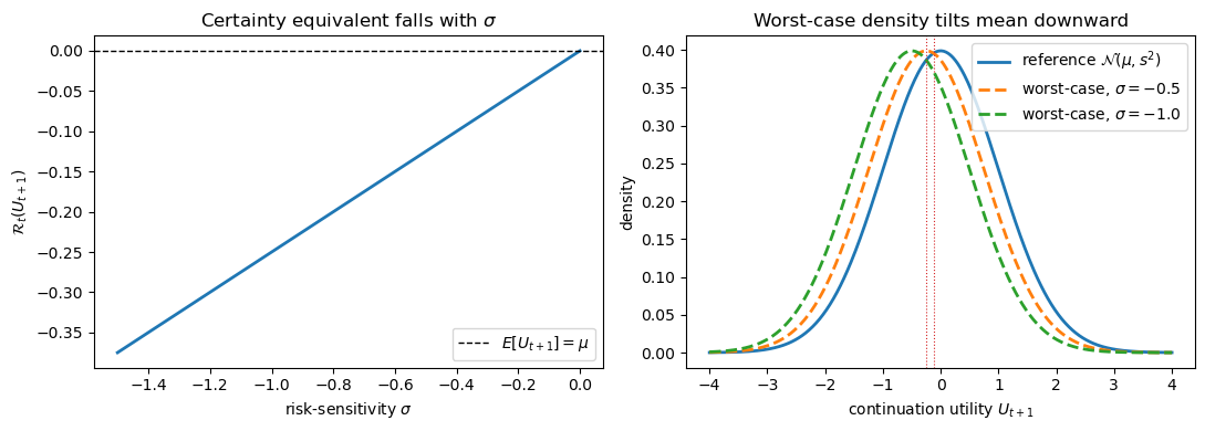
Fig. 77.1 Risk-sensitive operator and worst-case density#
The left panel shows the certainty equivalent \(\mathcal{R}_t\) sliding below the mean as \(\sigma\) becomes more negative.
The right panel shows the associated worst-case density of continuation utility: a robust agent behaves as if \(U_{t+1}\) were drawn from a pessimistically re-centered distribution (mean \(\mu + \frac{\sigma}{2}s^2\), dashed), while the operator value \(\mathcal{R}_t = \mu + \frac{\sigma}{4}s^2\) (dotted) sits halfway between it and the reference mean \(\mu\).
77.3. A preference for robustness#
The pessimistic tilt in the right panel above is not just an analogy.
[Hansen et al., 1999] show that the risk-sensitive problem is the value function of a two-player zero-sum game.
In this game, one player chooses the control \(\{i_t\}\) while a second, malevolent player chooses a distortion \(\{v_t\}\) to the conditional mean of the shocks.
The distorted law of motion is
The minimizing player would like to push the state in painful directions, but is restrained by a penalty on the size of the distortion.
With \(-1/\sigma \geq 0\) acting as a Lagrange multiplier on a constraint that bounds the distortion sequence, the Markov perfect equilibrium has value function
Because \(\sigma < 0\) makes \(-1/\sigma > 0\), the term \(-\frac{1}{\sigma}v'v\) penalizes the malevolent player for large distortions.
A smaller \(|1/\sigma|\) (more negative \(\sigma\)) means a cheaper distortion budget and hence a larger family of models the agent guards against — a stronger preference for robustness.
This is exactly the max-min expected utility structure of [Gilboa and Schmeidler, 1989]: the agent’s “nominal model” sets \(v_t = 0\), but they entertain a whole family of alternatives indexed by \(\{v_t\}\) and act against the worst case.
Following [Epstein and Wang, 1994], the non-uniqueness of the implied probability measures is a form of Knightian uncertainty.
The robust and risk-sensitive problems share the same value function matrix \(\Omega\) and the same decision rule \(i_t = -F x_t\); they differ only in interpretation.
77.4. The permanent income economy#
We now specialize to a habit-persistence version of the permanent income model.
A planner orders consumption streams \(\{c_t\}\) through a service stream \(\{s_t\}\) using the recursion
where \(\{b_t\}\) is an exogenous preference (bliss-point) shock.
Services are produced from consumption via the household technology
with \(\lambda > 0\) and \(\delta_h \in (0, 1)\).
Here \(h_t\) is a geometric average of current and past consumption, so (77.9) makes services depend negatively on a weighted average of past consumption — this is the habit persistence.
There is a linear production technology
and capital accumulates as \(k_t = \delta_k k_{t-1} + i_t\), where \(\{d_t\}\) is an exogenous endowment.
Combining,
so \(R\) is the gross physical return on capital, which in a decentralized economy equals the gross risk-free rate.
The endowment and preference shocks are driven by a common linear state,
This whole economy is a special case of the control problem (77.1)–(77.3): stack \(h_{t-1}\), \(k_{t-1}\), and \(z_t\) into the state \(x_t\) and let the control be \(i_t = s_t - b_t\).
77.4.1. The \(\sigma = 0\) benchmark and the martingale#
To build intuition, set \(\sigma = 0\) and impose the permanent income restriction \(\beta R = 1\), as in [Hall, 1978].
The first-order conditions then imply that the marginal utility of consumption services is a martingale,
and that \(\mu_{s,t}\) inherits the representation
for some loading vector \(v\).
Equation (77.13) is the classic statement that, under \(\beta R = 1\), consumption responds only to news — it is a random walk. This is the result that [Hall, 1978] and [Campbell, 1987] tested on aggregate U.S. data.
The scalar
measures the variance of the innovation to the marginal-utility martingale (77.14). It will be the one summary statistic of the benchmark economy that we need below.
Note
Under a rational-expectations reading, the benchmark \(\sigma = 0\) permanent income model has no precautionary savings, as emphasized by Zeldes. Introducing robustness (\(\sigma < 0\)) revives a precautionary motive: the consumer guards against worst-case mistakes in the conditional means of shocks.
77.5. Observational equivalence#
Here is the paper’s first headline result.
Proposition 77.1 (Observational Equivalence)
Fix all parameters except \(\beta\) and \(\sigma\). Suppose \(\beta R = 1\). There exists \(\underline{\sigma} < 0\) such that the optimal consumption–investment plan for \(\sigma = 0\) is also optimal for any \(\sigma \in (\underline{\sigma}, 0)\), provided the discount factor is lowered to a value \(\hat\beta(\sigma)\) that varies directly with \(\sigma\).
In words: as far as the quantities \(\{c_t, k_t\}\) are concerned, the robust (\(\sigma < 0\)) permanent income model is indistinguishable from the standard (\(\sigma = 0\)) one with a smaller discount factor.
Increasing the preference for robustness stimulates a precautionary motive for saving; lowering \(\beta\) makes saving less attractive; along a particular locus the two effects exactly cancel.
The proof is constructive and delivers an explicit locus of observationally equivalent \((\sigma, \hat\beta)\) pairs. Define
The equivalent discount factor \(\hat\beta\) solves
The lower bound \(\underline{\sigma}\) is the most negative \(\sigma\) for which the square root in (77.15) stays real.
Let’s reproduce the locus — a version of Figure 1 in [Hansen et al., 1999].
beta_bench = 0.9971         # benchmark discount factor (annual rate ~2.5%)
Rf = 1 / beta_bench         # gross risk-free return fixed by beta R = 1
theta2 = 0.01               # variance of the marginal-utility innovation, v'v

def Omega_scalar(beta, sigma, theta2):
    disc = (beta - 1 + sigma * theta2)**2 + 4 * sigma * theta2
    if disc < 0:
        return np.nan        # below sigma-underbar: no real solution
    return (beta - 1 + sigma * theta2 + np.sqrt(disc)) / (-2 * sigma * theta2)

def zeta_hat(beta, sigma, theta2):
    Om = Omega_scalar(beta, sigma, theta2)
    return 1 + (theta2 * sigma * Om) / (1 - sigma * theta2 * Om)

def beta_hat(sigma, theta2, Rf):
    "Discount factor that makes sigma observationally equivalent to sigma=0."
    if sigma == 0:
        return 1 / Rf
    f = lambda b: b * Rf * zeta_hat(b, sigma, theta2) - 1
    return brentq(f, 0.95, 1 / Rf - 1e-12)

sigmas = np.linspace(-1.2e-4, 0.0, 200)
betas = np.array([beta_hat(sg, theta2, Rf) for sg in sigmas])

fig, ax = plt.subplots(figsize=(7, 5))
ax.plot(betas, sigmas, lw=2)
ax.set_xlabel(r'discount factor $\hat\beta$')
ax.set_ylabel(r'risk-sensitivity $\sigma$')
ax.axhline(0, color='k', lw=0.8, ls='--')
plt.tight_layout()
plt.show()
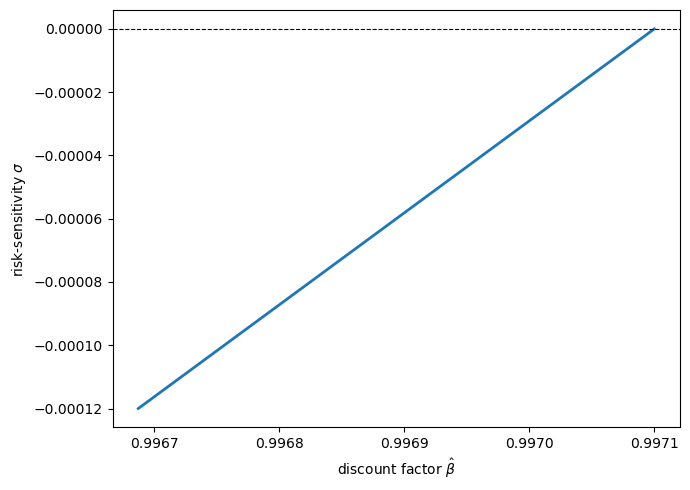
Fig. 77.2 Observationally equivalent \((\sigma, \hat\beta)\) pairs#
Every point on this curve generates exactly the same consumption and investment data.
Moving down the curve (more negative \(\sigma\), i.e. a stronger preference for robustness) requires a lower discount factor \(\hat\beta\) to keep quantities unchanged.
This is why consumption and savings data alone cannot tell us how much the consumer fears model misspecification.
77.6. Estimation#
Section 4 of [Hansen et al., 1999] turns the observational-equivalence result into an empirical strategy.
Because the quantity data cannot pin down \(\sigma\), the authors first estimate the \(\sigma = 0\) version of the model, conditioning the likelihood only on consumption and investment, and then use the locus of Proposition 77.1 to trace out the family of \((\sigma, \hat\beta)\) pairs consistent with those estimates.
Asset prices (the next section) break the tie.
77.6.1. The data and the likelihood#
The model is fit to U.S. post-war quarterly data, 1970:I–1996:III.
Consumption is measured as nondurables plus services.
Investment is measured as durables plus gross private investment.
Both series are deflated by the deterministic growth factor \(1.0033^{t}\), so the model is fit to detrended data.
The likelihood is Gaussian, built recursively (a Kalman filter), with the unobserved part of the initial state estimated using the methods of Hansen and Sargent.
77.6.2. Specification#
The preference shock is a constant, \(b_t = \mu_b\), fixed at \(\mu_b = 32\) — recall from (77.11)-discussion that the level of \(b_t\) does not affect the decision rules, only prices.
The endowment is the sum of a persistent and a transitory component, each a second-order autoregression driven by orthogonal shocks,
with \(d_t = \mu_d + d^{*}_t + \hat d_t\).
A likelihood comparison (a gain from AR(1) to AR(2) but not beyond) led the authors to a second-order specification for the transitory component.
The four parameters governing the endogenous dynamics are \((\gamma, \delta_k, \beta, \lambda)\).
The depreciation factor is set to \(\delta_k = 0.975\), and the permanent-income restriction \(\beta R = 1\) — confirmed by the unrestricted estimates — is imposed with \(\beta = 0.9971\), implying a \(2.5\%\) annual real interest rate after the growth adjustment.
The maximum-likelihood estimates (with habit persistence) are reproduced below — a version of Table 2 in [Hansen et al., 1999].
Parameter |
Symbol |
Estimate |
|---|---|---|
Discount factor |
\(\beta\) |
0.997 |
Habit depreciation |
\(\delta_h\) |
0.682 |
Habit weight |
\(\lambda\) |
2.443 |
Transitory AR roots |
\(\alpha_1, \alpha_2\) |
0.813, 0.189 |
Persistent AR roots |
\(\phi_1, \phi_2\) |
0.998, 0.704 |
Endowment mean |
\(\mu_d\) |
13.710 |
Transitory shock scale |
\(c_{\hat d}\) |
0.155 |
Persistent shock scale |
\(c_{d^{*}}\) |
0.108 |
The single most striking estimate is the autoregressive root \(\phi_1 = 0.998\) of the persistent endowment component — a number all but indistinguishable from a unit root.
77.6.3. Impulse responses and the permanent income mechanism#
The persistence of a shock is what determines how strongly consumption reacts to it.
Under the permanent income logic (with \(\beta R = 1\) and, for transparency, no habit), consumption jumps on impact by the annuity value of the change in wealth and is a martingale thereafter,
where \(\psi_j = \partial d_{t+j} / \partial w_t\) is the endowment’s own impulse response.
A near-permanent shock has a large present value and moves consumption a lot; a transitory shock has a small present value and barely moves it.
Let’s compute the endowment responses (77.18)–(77.19) and the implied consumption responses.
def ar2_irf(r1, r2, c, H):
    "Impulse response of (1 - r1 L)(1 - r2 L) x = c w to a unit w shock."
    psi = np.zeros(H)
    psi[0] = c
    if H > 1:
        psi[1] = (r1 + r2) * psi[0]
    for j in range(2, H):
        psi[j] = (r1 + r2) * psi[j-1] - r1 * r2 * psi[j-2]
    return psi

H = 50
disc = Rf**(-np.arange(H))                      # Rf = 1/beta from the previous cell

psi_p = ar2_irf(0.998, 0.704, 0.108, H)         # persistent endowment d*
psi_t = ar2_irf(0.813, 0.189, 0.155, H)         # transitory endowment d_hat

# permanent income consumption response: a flat (martingale) jump
dc_p = (1 - 1/Rf) * np.sum(disc * psi_p)
dc_t = (1 - 1/Rf) * np.sum(disc * psi_t)

print(f"persistent shock: consumption responds to "
      f"{100*dc_p/psi_p[0]:.0f}% of the impact")
print(f"transitory shock: consumption responds to "
      f"{100*dc_t/psi_t[0]:.0f}% of the impact")

fig, axes = plt.subplots(1, 2, figsize=(11, 4), sharey=True)
for ax, psi, dc, title in [
        (axes[0], psi_p, dc_p, 'Persistent endowment shock $d^{*}$'),
        (axes[1], psi_t, dc_t, 'Transitory endowment shock $\\hat d$')]:
    ax.plot(psi, lw=2, label='endowment response $\\psi_j$')
    ax.axhline(dc, color='C3', ls='--', lw=2, label='consumption response $\\Delta c$')
    ax.set_xlabel('horizon $j$ (quarters)')
    ax.set_title(title)
    ax.legend()
axes[0].set_ylabel('response')
plt.tight_layout()
plt.show()
persistent shock: consumption responds to 41% of the impact
transitory shock: consumption responds to 2% of the impact
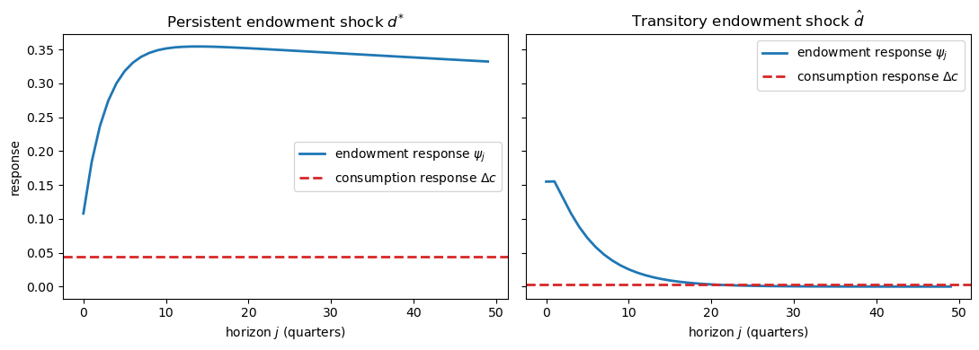
Fig. 77.3 Endowment and consumption impulse responses#
The contrast is the heart of the permanent income hypothesis tested by [Hall, 1978] and [Campbell, 1987].
Consumption tracks a large fraction of the persistent shock — whose near-unit root makes it almost permanent income — but only a sliver of the transitory shock, the bulk of which is saved and shows up as investment.
Note
With habit persistence (\(\lambda > 0\)) the consumption responses are no longer flat: they become hump-shaped, because services rather than consumption obey the martingale logic. The estimated \(\lambda = 2.443\) and \(\delta_h = 0.682\) imply economically important habit effects, and a likelihood-ratio comparison strongly rejects \(\lambda = 0\). [Hansen et al., 1999] compare these magnitudes with the habit estimates in the time-nonseparable preference literature.
77.7. Asset pricing and the market price of risk#
Section 5 of [Hansen et al., 1999] shows how the observationally-equivalent pairs that look identical in quantity data have different implications for asset prices.
77.7.1. Decentralization#
Following [Lucas, 1978], we regard the robust (or risk-sensitive) planning solution as the allocation of a competitive economy populated by a large number of identical agents who trade securities.
Equilibrium prices are the shadow prices that leave each agent content to consume the planner’s allocation, treating it as an endowment process.
The equilibrium law of motion for the state is
and the value function at the optimum is \(U^{e}_t = x_t' \Omega x_t + \rho\).
To support the robust allocation, prices must be computed using the same pessimistic, distorted beliefs that rationalize the planner’s choices.
This is where risk-sensitivity (\(\sigma < 0\)) leaves its fingerprint on prices even though, by observational equivalence, it leaves no trace in quantities.
77.7.2. The twisting operator and distorted beliefs#
Pricing a claim to next period’s utility is trivial under the von Neumann–Morgenstern specification but nontrivial under risk-sensitivity.
The key object is the twisting operator
which re-weights outcomes by the exponential of equilibrium continuation utility.
It satisfies the subgradient inequality
so \(\mathcal{T}_t\) behaves like a distorted conditional expectation — exactly the change of measure used to price derivative claims in [Epstein and Wang, 1994].
Concretely, \(\mathcal{T}_t\) is the ordinary conditional expectation under a distorted transition law
with \(\hat A\) given by (77.30)-style risk corrections.
Because \(\sigma < 0\) and \(\Omega\) is negative semidefinite, \((I - \sigma C'\Omega C)^{-1}\) exceeds the identity: the pricing measure assigns a pessimistically shifted conditional mean and an inflated conditional variance to next period’s state.
These two distortions are precisely what generate risk premia.
77.7.3. Multi-period claims and the one-period stochastic discount factor#
Prices of streams are built by iterating the operator.
Define \(\mathcal{S}_{t,\tau} = \mathcal{T}_t \mathcal{T}_{t+1} \cdots \mathcal{T}_{t+\tau-1}\). The time-\(t\) price of a claim to the consumption stream \(\{c_{t+\tau}\}\) is then a discounted sum of twisted marginal utilities, and the one-period security with payoff \(p_{t+1}\) is priced as
where \(\mathcal{M}^{c}_t\) is the marginal utility of consumption and \(m_{t+1,t}\) is the one-period stochastic discount factor (intertemporal marginal rate of substitution).
Under risk-sensitivity, \(m_{t+1,t}\) factors into two pieces,
where
is the familiar intertemporal marginal rate of substitution (the only term present when \(\sigma = 0\)), and
is a multiplicative adjustment with conditional mean one. The factor (77.27) is the source of the extra risk premia.
77.7.4. The market price of risk#
Under the robustness interpretation, the same multiplicative factor equals a likelihood ratio between the worst-case and reference shock densities,
where \(\hat v_t\) is the worst-case conditional-mean distortion chosen by the malevolent player.
A direct calculation gives
so that, for small distortions,
The market price of risk — the maximal Sharpe ratio attainable, equal to \(\operatorname{std}_t(m_{t+1,t}) / \mathbb{E}_t(m_{t+1,t})\) along the efficient frontier (the [Hansen and Jagannathan, 1991] bound) — is therefore approximately equal to the magnitude of the worst-case distortion \(|\hat v_t|\).
This is the paper’s punchline: a conditional-mean misspecification of \(x\%\) of a unit-norm direction raises the market price of risk by roughly \(x/100\).
A small, statistically-hard-to-detect doubt about the model can generate the large price of risk seen in the data.
Let’s check the key identity (77.29) by Monte Carlo.
rng = np.random.default_rng(12345)

def mpr_check(v_hat, n=2_000_000):
    """
    Simulate the worst-case likelihood ratio m^u and compare its
    conditional standard deviation to |v_hat|.
    """
    k = len(v_hat)
    w = rng.standard_normal((n, k))
    # log likelihood ratio of N(v_hat, I) relative to N(0, I)
    log_mu = w @ v_hat - 0.5 * v_hat @ v_hat
    mu = np.exp(log_mu)
    return mu.mean(), mu.std(), np.linalg.norm(v_hat)

print(f"{'|v_hat|':>10}{'E[m^u]':>12}{'std(m^u)':>12}{'approx |v_hat|':>16}")
for scale in [0.05, 0.10, 0.20]:
    v_hat = np.array([scale, 0.0])      # distortion in one direction
    mean, std, norm_v = mpr_check(v_hat)
    print(f"{norm_v:10.3f}{mean:12.4f}{std:12.4f}{norm_v:16.3f}")
   |v_hat|      E[m^u]    std(m^u)  approx |v_hat|
     0.050      1.0000      0.0500           0.050
     0.100      0.9999      0.1003           0.100
     0.200      0.9997      0.2022           0.200
The simulated conditional mean of \(m^{u}\) is one, and its conditional standard deviation tracks \(|\hat v_t|\) closely — confirming (77.29).
A 10% distortion delivers a market price of risk near 0.10.
77.8. A risk-sensitive regulator#
To see the robust decision rules and worst-case shocks concretely, we solve the recursive risk-sensitive control problem (77.1)–(77.3) directly.
Guess a value function \(W(x) = x' \Omega x + \rho\) with \(\Omega\) negative semidefinite. The risk-sensitive operator (77.4) acting on this quadratic form introduces the risk adjustment
so that, replacing \(\Omega\) by \(\mathcal{D}(\Omega)\), the Bellman equation becomes an ordinary linear-quadratic one.
Iterating
to a fixed point yields the optimal rule \(i_t = -F x_t\).
The worst-case mean distortion is then linear in the state, \(\hat v_t = G x_t\), with
When \(\sigma = 0\) we have \(\mathcal{D}(\Omega) = \Omega\) and \(G = 0\), recovering the standard regulator.
def solve_rslq(A, B, C, Q, R, beta, sigma, N=None,
               tol=1e-12, max_iter=100_000):
    """
    Solve the recursive risk-sensitive LQ problem

        U_t = -(x'R x + i'Q i + 2 i'N x) + beta R_t(U_{t+1})
        x_{t+1} = A x_t + B i_t + C w_{t+1}

    Returns the feedback rule F (i = -F x), the value matrix Omega,
    the closed-loop matrix A - B F, and the worst-case loading G (v = G x).
    """
    A, B, C, Q, R = map(np.atleast_2d, (A, B, C, Q, R))
    n, kw = A.shape[0], C.shape[1]
    if N is None:
        N = np.zeros((B.shape[1], n))
    Omega = -np.eye(n)                # negative-definite start
    Iw = np.eye(kw)
    for it in range(max_iter):
        M = Iw - sigma * C.T @ Omega @ C
        D = Omega + sigma * Omega @ C @ np.linalg.solve(M, C.T @ Omega)
        F = np.linalg.solve(Q - beta * B.T @ D @ B, N - beta * B.T @ D @ A)
        Acl = A - B @ F
        Omega_new = (-R - F.T @ Q @ F + (F.T @ N + N.T @ F)
                     + beta * Acl.T @ D @ Acl)
        if np.max(np.abs(Omega_new - Omega)) < tol:
            Omega = Omega_new
            break
        Omega = Omega_new
    M = Iw - sigma * C.T @ Omega @ C
    G = sigma * np.linalg.solve(M, C.T @ Omega @ (A - B @ F))
    return F, Omega, A - B @ F, G
We first verify that at \(\sigma = 0\) our solver reproduces QuantEcon’s ordinary LQ regulator.
# a stylized stable regulator with a persistent shock
A = np.array([[0.9, 0.0],
              [0.0, 0.8]])
B = np.array([[1.0],
              [0.0]])
C = np.array([[0.3],
              [0.2]])
Q = np.array([[1.0]])
R = np.eye(2)
beta = 0.95

# QuantEcon ordinary LQ
lq = qe.LQ(Q, R, A, B, C=C, beta=beta)
P, F_qe, d = lq.stationary_values()

# our solver at sigma = 0
F0, Omega0, Acl0, G0 = solve_rslq(A, B, C, Q, R, beta, sigma=0.0)

print("QuantEcon LQ feedback rule F :", F_qe.flatten())
print("solve_rslq  feedback rule F  :", F0.flatten())
print("max |difference|             :", np.max(np.abs(F0 - F_qe)))
QuantEcon LQ feedback rule F : [0.52479699 0.        ]
solve_rslq  feedback rule F  : [0.52479699 0.        ]
max |difference|             : 1.1102230246251565e-16
The two agree to machine precision.
Now we crank up the preference for robustness and inspect how the control rule and the worst-case shock respond.
sigmas = [0.0, -0.3, -0.6]

print(f"{'sigma':>7}{'F[0]':>10}{'F[1]':>10}{'G[0]':>10}{'G[1]':>10}")
for sigma in sigmas:
    F, Omega, Acl, G = solve_rslq(A, B, C, Q, R, beta, sigma)
    print(f"{sigma:7.2f}{F[0,0]:10.4f}{F[0,1]:10.4f}{G[0,0]:10.4f}{G[0,1]:10.4f}")
  sigma      F[0]      F[1]      G[0]      G[1]
   0.00    0.5248    0.0000   -0.0000   -0.0000
  -0.30    0.5357    0.0340    0.0532    0.1370
  -0.60    0.5490    0.0803    0.1154    0.3169
As \(\sigma\) becomes more negative:
the feedback gain \(F\) grows — the robust agent reacts more aggressively to the state, since it fears the worst-case shock will amplify deviations;
the worst-case loading \(G\) moves away from zero — the malevolent player pushes the shock in the direction that hurts most.
Finally, let’s see the worst-case distortion in action by simulating the controlled state under the reference model while displaying the conditional mean distortion \(\hat v_t = G x_t\) the robust agent is guarding against.
def simulate(A, B, C, F, G, T=60, seed=0):
    rng = np.random.default_rng(seed)
    n, kw = A.shape[0], C.shape[1]
    x = np.zeros((T + 1, n))
    v = np.zeros((T, kw))
    x[0] = np.array([1.0, 1.0])          # initial deviation
    for t in range(T):
        v[t] = (G @ x[t]).flatten()
        w = rng.standard_normal(kw)
        x[t + 1] = A @ x[t] + (B @ (-F @ x[t])).flatten() + (C @ w).flatten()
    return x, v

fig, axes = plt.subplots(1, 2, figsize=(11, 4))

for sigma, color in zip([0.0, -0.6], ['C0', 'C3']):
    F, Omega, Acl, G = solve_rslq(A, B, C, Q, R, beta, sigma)
    x, v = simulate(A, B, C, F, G, seed=42)
    axes[0].plot(x[:, 0], color=color, lw=2, label=f'$\\sigma={sigma}$')
    axes[1].plot(v[:, 0], color=color, lw=2, label=f'$\\sigma={sigma}$')

axes[0].set_title('Controlled state $x_{1,t}$')
axes[0].set_xlabel('$t$')
axes[0].axhline(0, color='k', lw=0.8, ls='--')
axes[0].legend()

axes[1].set_title(r'Worst-case mean distortion $\hat v_{1,t}$')
axes[1].set_xlabel('$t$')
axes[1].axhline(0, color='k', lw=0.8, ls='--')
axes[1].legend()

plt.tight_layout()
plt.show()

Fig. 77.4 Controlled state and worst-case distortion#
For \(\sigma = 0\) the distortion is identically zero — the agent fully trusts the model.
For \(\sigma < 0\) the robust agent’s decisions are shaped by a nonzero worst-case distortion that feeds back on the state, exactly the mechanism that — through (77.29) — inflates the market price of risk.
77.9. Exercises#
Exercise 77.1
The Gaussian formula (77.5) says that for \(U_{t+1} \sim \mathcal{N}(\mu, s^2)\),
Derive this result directly from the definition (77.4).
Hint: use the moment generating function of a normal random variable, \(\mathbb{E}[\exp(a U)] = \exp(a\mu + a^2 s^2 / 2)\).
Solution
Start from the definition with \(a = \sigma/2\):
Since \(U_{t+1} \sim \mathcal{N}(\mu, s^2)\), the moment generating function gives
Taking logs and multiplying by \(2/\sigma\),
Letting \(\sigma \to 0\) recovers \(\mathcal{R}_t(U_{t+1}) = \mu = \mathbb{E}_t U_{t+1}\), as expected.
Exercise 77.2
The observational-equivalence locus has a left endpoint \(\underline{\sigma}\): the most negative \(\sigma\) for which (77.15) has a real solution.
Using the code from the lecture, find \(\underline{\sigma}\) numerically for theta2 = 0.01 and for theta2 = 0.02, and explain why a larger \(\theta^2\) shrinks the admissible range of \(\sigma\).
Hint: the square root is real when the discriminant \((\beta - 1 + \sigma\theta^2)^2 + 4\sigma\theta^2 \geq 0\), evaluated at the relevant \(\hat\beta\).
Solution
The boundary \(\underline{\sigma}\) is the most negative \(\sigma\) at which a valid \(\hat\beta\) can still be found. We scan \(\sigma\) downward and stop when beta_hat can no longer return a real solution.
def sigma_underbar(theta2, Rf, grid=np.linspace(-1e-6, -5e-4, 5000)):
    last_ok = 0.0
    for sg in grid:
        try:
            b = beta_hat(sg, theta2, Rf)
            if np.isnan(Omega_scalar(b, sg, theta2)):
                break
            last_ok = sg
        except ValueError:
            break
    return last_ok

for theta2 in [0.01, 0.02]:
    sb = sigma_underbar(theta2, Rf)
    print(f"theta2 = {theta2}:  sigma_underbar ≈ {sb:.3e}")
theta2 = 0.01:  sigma_underbar ≈ -2.105e-04
theta2 = 0.02:  sigma_underbar ≈ -1.052e-04
A larger \(\theta^2\) means the marginal-utility martingale (77.14) carries a bigger innovation variance, so each unit of \(|\sigma|\) generates a larger risk adjustment. The discriminant in (77.15), which contains the term \(4\sigma\theta^2 < 0\), turns negative at a smaller \(|\sigma|\). Hence the admissible range \((\underline{\sigma}, 0)\) shrinks as \(\theta^2\) grows.
Exercise 77.3
The market-price-of-risk approximation (77.29) states that \(\operatorname{std}_t(m^u_{t+1,t}) = [\exp(\hat v_t'\hat v_t) - 1]^{1/2} \approx |\hat v_t|\).
For the risk-sensitive regulator solved in the lecture (with \(A\), \(B\), \(C\), \(Q\), \(R\), \(\beta\) as given there), compute the exact market price of risk \([\exp(\hat v_t' \hat v_t) - 1]^{1/2}\) as a function of \(\sigma\), evaluated at the state \(x = (1, 1)'\), and plot it together with the linear approximation \(|\hat v_t|\).
Comment on the range of \(\sigma\) over which the approximation is accurate.
Solution
We solve the regulator for a grid of \(\sigma\) values, evaluate \(\hat v_t = G x\) at \(x = (1,1)'\), and compare the exact and approximate market prices of risk.
x_eval = np.array([1.0, 1.0])
sigma_grid = np.linspace(-1.0, 0.0, 80)

exact, approx = [], []
for sigma in sigma_grid:
    F, Omega, Acl, G = solve_rslq(A, B, C, Q, R, beta, sigma)
    v_hat = (G @ x_eval).flatten()
    nv2 = v_hat @ v_hat
    exact.append(np.sqrt(np.exp(nv2) - 1))
    approx.append(np.sqrt(nv2))           # |v_hat|

fig, ax = plt.subplots(figsize=(7, 5))
ax.plot(sigma_grid, exact, lw=2, label=r'exact $[\exp(\hat v\,\!^\prime \hat v)-1]^{1/2}$')
ax.plot(sigma_grid, approx, lw=2, ls='--', label=r'approximation $|\hat v|$')
ax.set_xlabel(r'risk-sensitivity $\sigma$')
ax.set_ylabel('market price of risk')
ax.set_title('exact vs. approximate market price of risk')
ax.legend()
plt.tight_layout()
plt.show()
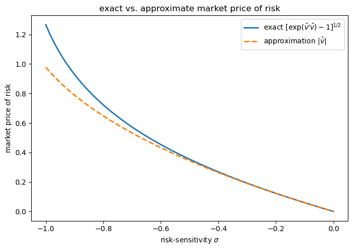
The two curves are nearly indistinguishable for small \(|\hat v_t|\) (i.e. \(\sigma\) close to zero) because \(\exp(z) - 1 \approx z\) when \(z\) is small.
They separate only when the preference for robustness — and hence the worst-case distortion — becomes large.
This is precisely the regime [Hansen et al., 1999] emphasize: small, hard-to-detect distortions map almost linearly into the market price of risk.