87. Markov Perfect Equilibrium#
In addition to what’s in Anaconda, this lecture will need the following libraries:
!pip install quantecon
87.1. Overview#
This lecture describes the concept of Markov perfect equilibrium.
Markov perfect equilibrium is a key notion for analyzing economic problems involving dynamic strategic interaction, and a cornerstone of applied game theory.
In this lecture, we teach Markov perfect equilibrium by example.
We will focus on settings with
two players
quadratic payoff functions
linear transition rules for the state
Other references include chapter 7 of [Ljungqvist and Sargent, 2018].
Let’s start with some standard imports:
import matplotlib.pyplot as plt
import numpy as np
import quantecon as qe
87.2. Background#
Markov perfect equilibrium is a refinement of the concept of Nash equilibrium.
It is used to study settings where multiple decision-makers interact non-cooperatively over time, each pursuing its own objective.
The agents in the model face a common state vector, the time path of which is influenced by – and influences – their decisions.
In particular, the transition law for the state that confronts each agent is affected by decision rules of other agents.
Individual payoff maximization requires that each agent solve a dynamic programming problem that includes this transition law.
Markov perfect equilibrium prevails when no agent wishes to revise its policy, taking as given the policies of all other agents.
Well known examples include
Choice of price, output, location or capacity for firms in an industry (e.g., [Ericson and Pakes, 1995], [Ryan, 2012], [Doraszelski and Satterthwaite, 2010]).
Rate of extraction from a shared natural resource, such as a fishery (e.g., [Levhari and Mirman, 1980], [Van Long, 2011]).
Let’s examine a model of the first type.
87.2.1. Example: A Duopoly Model#
Two firms are the only producers of a good, the demand for which is governed by a linear inverse demand function
Here \(p = p_t\) is the price of the good, \(q_i = q_{it}\) is the output of firm \(i=1,2\) at time \(t\) and \(a_0 > 0, a_1 >0\).
In (87.1) and what follows,
the time subscript is suppressed when possible to simplify notation
\(\hat x\) denotes a next period value of variable \(x\)
Each firm recognizes that its output affects total output and therefore the market price.
The one-period payoff function of firm \(i\) is price times quantity minus adjustment costs:
Substituting the inverse demand curve (87.1) into (87.2) lets us express the one-period payoff as
where \(q_{-i}\) denotes the output of the firm other than \(i\).
The objective of the firm is to maximize \(\sum_{t=0}^\infty \beta^t \pi_{it}\).
Firm \(i\) chooses a decision rule that sets next period quantity \(\hat q_i\) as a function \(f_i\) of the current state \((q_i, q_{-i})\).
An essential aspect of a Markov perfect equilibrium is that each firm takes the decision rule of the other firm as known and given.
Given \(f_{-i}\), the Bellman equation of firm \(i\) is
Definition 87.1 (Markov Perfect Equilibrium)
A Markov perfect equilibrium of the duopoly model is a pair of value functions \((v_1, v_2)\) and a pair of policy functions \((f_1, f_2)\) such that, for each \(i \in \{1, 2\}\) and each possible state,
The value function \(v_i\) satisfies Bellman equation (87.4).
The maximizer on the right side of (87.4) equals \(f_i(q_i, q_{-i})\).
The adjective “Markov” denotes that the equilibrium decision rules depend only on the current values of the state variables, not other parts of their histories.
“Perfect” means complete, in the sense that the equilibrium is constructed by backward induction and hence builds in optimizing behavior for each firm at all possible future states.
These include many states that will not be reached when we iterate forward on the pair of equilibrium strategies \(f_i\) starting from a given initial state.
87.2.2. Computation#
One strategy for computing a Markov perfect equilibrium is iterating to convergence on pairs of Bellman equations and decision rules.
In particular, let \(v_i^j,f_i^j\) be the value function and policy function for firm \(i\) at the \(j\)-th iteration.
Imagine constructing the iterates
These iterations can be challenging to implement computationally.
However, they simplify for the case in which one-period payoff functions are quadratic and transition laws are linear — which takes us to our next topic.
87.3. Linear Markov Perfect Equilibria#
As we saw in the duopoly example, the study of Markov perfect equilibria in games with two players leads us to an interrelated pair of Bellman equations.
In linear-quadratic dynamic games, these “stacked Bellman equations” become “stacked Riccati equations” with a tractable mathematical structure.
We’ll lay out that structure in a general setup and then apply it to some simple problems.
87.3.1. Coupled Linear Regulator Problems#
We consider a general linear-quadratic regulator game with two players.
For convenience, we’ll start with a finite horizon formulation, where \(t_0\) is the initial date and \(t_1\) is the common terminal date.
Player \(i\) takes \(\{u_{-it}\}\) as given and minimizes
while the state evolves according to
Here
\(x_t\) is an \(n \times 1\) state vector and \(u_{it}\) is a \(k_i \times 1\) vector of controls for player \(i\)
\(R_i\) is \(n \times n\)
\(S_i\) is \(k_{-i} \times k_{-i}\)
\(Q_i\) is \(k_i \times k_i\)
\(W_i\) is \(n \times k_i\)
\(M_i\) is \(k_{-i} \times k_i\)
\(A\) is \(n \times n\)
\(B_i\) is \(n \times k_i\)
87.3.2. Computing Equilibrium#
We formulate a linear Markov perfect equilibrium as follows.
Player \(i\) employs linear decision rules \(u_{it} = - F_{it} x_t\), where \(F_{it}\) is a \(k_i \times n\) matrix.
A Markov perfect equilibrium is a pair of sequences \(\{F_{1t}, F_{2t}\}\) over \(t = t_0, \ldots, t_1 - 1\) such that
\(\{F_{1t}\}\) solves player 1’s problem, taking \(\{F_{2t}\}\) as given, and
\(\{F_{2t}\}\) solves player 2’s problem, taking \(\{F_{1t}\}\) as given
If we take \(u_{2t} = - F_{2t} x_t\) and substitute it into (87.6) and (87.7), then player 1’s problem becomes minimization of
subject to
where
\(\Lambda_{it} := A - B_{-i} F_{-it}\)
\(\Pi_{it} := R_i + F_{-it}' S_i F_{-it}\)
\(\Gamma_{it} := W_i' - M_i' F_{-it}\)
This is an LQ dynamic programming problem that can be solved by working backwards.
Decision rules that solve this problem are
where \(P_{1t}\) solves the matrix Riccati difference equation
Similarly, decision rules that solve player 2’s problem are
where \(P_{2t}\) solves
Here, in all cases \(t = t_0, \ldots, t_1 - 1\) and the terminal conditions are \(P_{it_1} = 0\).
The solution procedure is to use equations (87.10), (87.11), (87.12), and (87.13), and “work backwards” from time \(t_1 - 1\).
Since we’re working backward, \(P_{1t+1}\) and \(P_{2t+1}\) are taken as given at each stage.
Moreover, since
some terms on the right-hand side of (87.10) contain \(F_{2t}\)
some terms on the right-hand side of (87.12) contain \(F_{1t}\)
we need to solve these \(k_1 + k_2\) equations simultaneously.
87.3.2.1. Key Insight#
A key insight is that equations (87.10) and (87.12) are linear in \(F_{1t}\) and \(F_{2t}\).
After these equations have been solved, we can take \(F_{it}\) and solve for \(P_{it}\) in (87.11) and (87.13).
87.3.2.2. Infinite Horizon#
We often want to compute the solutions of such games for infinite horizons, in the hope that the decision rules \(F_{it}\) settle down to be time-invariant as \(t_1 \rightarrow +\infty\).
In practice, we usually fix \(t_1\) and compute the equilibrium of an infinite horizon game by driving \(t_0 \rightarrow - \infty\).
This is the approach we adopt in the next section.
87.3.3. Implementation#
We use the function nnash from QuantEcon.py that computes a Markov perfect equilibrium of the infinite horizon linear-quadratic dynamic game in the manner described above.
87.4. Application#
Let’s use these procedures to treat some applications, starting with the duopoly model.
87.4.1. A Duopoly Model#
To map the duopoly model into coupled linear-quadratic dynamic programming problems, define the state and controls as
If we write
where \(Q_1 = Q_2 = \gamma\),
then we recover the one-period payoffs in expression (87.3).
The law of motion for the state \(x_t\) is \(x_{t+1} = A x_t + B_1 u_{1t} + B_2 u_{2t}\) where
The optimal decision rule of firm \(i\) will take the form \(u_{it} = - F_i x_t\), inducing the following closed-loop system for the evolution of \(x\) in the Markov perfect equilibrium:
87.4.2. Parameters and Solution#
Consider the previously presented duopoly model with parameter values of:
\(a_0 = 10\)
\(a_1 = 2\)
\(\beta = 0.96\)
\(\gamma = 12\)
From these, we compute the infinite horizon MPE using the preceding code
import numpy as np
import quantecon as qe

# Parameters
a0 = 10.0
a1 = 2.0
β = 0.96
γ = 12.0

# In LQ form
A = np.eye(3)
B1 = np.array([[0.], [1.], [0.]])
B2 = np.array([[0.], [0.], [1.]])


R1 = [[      0.,     -a0 / 2,          0.],
      [-a0 / 2.,          a1,     a1 / 2.],
      [       0,     a1 / 2.,          0.]]

R2 = [[     0.,           0.,      -a0 / 2],
      [     0.,           0.,      a1 / 2.],
      [-a0 / 2,      a1 / 2.,           a1]]

Q1 = Q2 = γ
S1 = S2 = W1 = W2 = M1 = M2 = 0.0

# Solve using QE's nnash function
F1, F2, P1, P2 = qe.nnash(A, B1, B2, R1, R2, Q1,
                          Q2, S1, S2, W1, W2, M1,
                          M2, beta=β)

# Display policies
print("Computed policies for firm 1 and firm 2:\n")
print(f"F1 = {F1}")
print(f"F2 = {F2}")
print("\n")
Computed policies for firm 1 and firm 2:

F1 = [[-0.66846615  0.29512482  0.07584666]]
F2 = [[-0.66846615  0.07584666  0.29512482]]
Running the code produces the following output.
One way to see that \(F_i\) is indeed optimal for firm \(i\) taking \(F_2\) as given is to use QuantEcon.py’s LQ class.
In particular, let’s take F2 as computed above, plug it into (87.8) and (87.9) to get firm 1’s problem and solve it using LQ.
We hope that the resulting policy will agree with F1 as computed above
Λ1 = A - B2 @ F2
lq1 = qe.LQ(Q1, R1, Λ1, B1, beta=β)
P1_ih, F1_ih, d = lq1.stationary_values()
F1_ih
array([[-0.66846613, 0.29512482, 0.07584666]])
This is close enough for rock and roll, as they say in the trade.
Indeed, np.allclose agrees with our assessment
np.allclose(F1, F1_ih)
True
87.4.3. Dynamics#
Let’s now investigate the dynamics of price and output in this simple duopoly model under the MPE policies.
Given our optimal policies \(F1\) and \(F2\), the state evolves according to (87.14).
The following program
imports \(F1\) and \(F2\) from the previous program along with all parameters.
computes the evolution of \(x_t\) using (87.14).
extracts and plots industry output \(q_t = q_{1t} + q_{2t}\) and price \(p_t = a_0 - a_1 q_t\).
AF = A - B1 @ F1 - B2 @ F2
n = 20
x = np.empty((3, n))
x[:, 0] = 1, 1, 1
for t in range(n-1):
    x[:, t+1] = AF @ x[:, t]
q1 = x[1, :]
q2 = x[2, :]
q = q1 + q2       # Total output, MPE
p = a0 - a1 * q   # Price, MPE

fig, ax = plt.subplots(figsize=(9, 5.8))
ax.plot(q, 'b-', lw=2, alpha=0.75, label='total output')
ax.plot(p, 'g-', lw=2, alpha=0.75, label='price')
ax.set_title('Output and prices, duopoly MPE')
ax.legend(frameon=False)
plt.show()
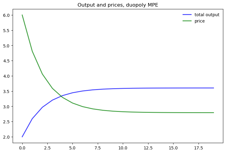
Note that the initial condition has been set to \(q_{10} = q_{20} = 1.0\).
To gain some perspective we can compare this to what happens in the monopoly case.
The first panel in the next figure compares output of the monopolist and industry output under the MPE, as a function of time.
The second panel shows analogous curves for price.
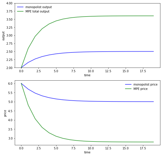
Here parameters are the same as above for both the MPE and monopoly solutions.
The monopolist initial condition is \(q_0 = 2.0\) to mimic the industry initial condition \(q_{10} = q_{20} = 1.0\) in the MPE case.
As expected, output is higher and prices are lower under duopoly than monopoly.
87.5. Exercises#
Exercise 87.1
Replicate the pair of figures showing the comparison of output and prices for the monopolist and duopoly under MPE.
Parameters are as in duopoly_mpe.py and you can use that code to compute MPE policies under duopoly.
The optimal policy in the monopolist case can be computed using QuantEcon.py’s LQ class.
Solution
First, let’s compute the duopoly MPE under the stated parameters
# == Parameters == #
a0 = 10.0
a1 = 2.0
β = 0.96
γ = 12.0

# == In LQ form == #
A  = np.eye(3)
B1 = np.array([[0.], [1.], [0.]])
B2 = np.array([[0.], [0.], [1.]])
R1 = [[      0.,      -a0/2,          0.],
      [-a0 / 2.,         a1,     a1 / 2.],
      [       0,    a1 / 2.,          0.]]

R2 = [[     0.,          0.,     -a0 / 2],
      [     0.,          0.,     a1 / 2.],
      [-a0 / 2,     a1 / 2.,          a1]]

Q1 = Q2 = γ
S1 = S2 = W1 = W2 = M1 = M2 = 0.0

# == Solve using QE's nnash function == #
F1, F2, P1, P2 = qe.nnash(A, B1, B2, R1, R2, Q1,
                          Q2, S1, S2, W1, W2, M1,
                          M2, beta=β)
Now we evaluate the time path of industry output and prices given initial condition \(q_{10} = q_{20} = 1\).
AF = A - B1 @ F1 - B2 @ F2
n = 20
x = np.empty((3, n))
x[:, 0] = 1, 1, 1
for t in range(n-1):
    x[:, t+1] = AF @ x[:, t]
q1 = x[1, :]
q2 = x[2, :]
q = q1 + q2       # Total output, MPE
p = a0 - a1 * q   # Price, MPE
Next, let’s have a look at the monopoly solution.
For the state and control, we take
To convert to an LQ problem we set
in the payoff function \(x_t' R x_t + u_t' Q u_t\) and
in the law of motion \(x_{t+1} = A x_t + B u_t\).
We solve for the optimal policy \(u_t = - Fx_t\) and track the resulting dynamics of \(\{q_t\}\), starting at \(q_0 = 2.0\).
R = a1
Q = γ
A = B = 1
lq_alt = qe.LQ(Q, R, A, B, beta=β)
P, F, d = lq_alt.stationary_values()
q_bar = a0 / (2.0 * a1)
qm = np.empty(n)
qm[0] = 2
x0 = qm[0] - q_bar
x = x0
for i in range(1, n):
    x = A * x - B * F * x
    qm[i] = float(x.item()) + q_bar
pm = a0 - a1 * qm
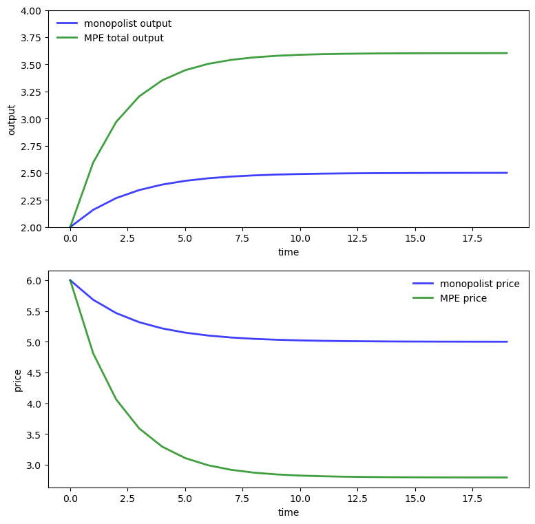
Let’s have a look at the different time paths
fig, axes = plt.subplots(2, 1, figsize=(9, 9))

ax = axes[0]
ax.plot(qm, 'b-', lw=2, alpha=0.75, label='monopolist output')
ax.plot(q, 'g-', lw=2, alpha=0.75, label='MPE total output')
ax.set(ylabel="output", xlabel="time", ylim=(2, 4))
ax.legend(loc='upper left', frameon=0)

ax = axes[1]
ax.plot(pm, 'b-', lw=2, alpha=0.75, label='monopolist price')
ax.plot(p, 'g-', lw=2, alpha=0.75, label='MPE price')
ax.set(ylabel="price", xlabel="time")
ax.legend(loc='upper right', frameon=0)
plt.show()
Exercise 87.2
In this exercise, we consider a slightly more sophisticated duopoly problem.
It takes the form of infinite horizon linear-quadratic game proposed by Judd [Judd, 1990].
Two firms set prices and quantities of two goods interrelated through their demand curves.
Relevant variables are defined as follows:
\(I_{it}\) = inventories of firm \(i\) at beginning of \(t\)
\(q_{it}\) = production of firm \(i\) during period \(t\)
\(p_{it}\) = price charged by firm \(i\) during period \(t\)
\(S_{it}\) = sales made by firm \(i\) during period \(t\)
\(E_{it}\) = costs of production of firm \(i\) during period \(t\)
\(C_{it}\) = costs of carrying inventories for firm \(i\) during \(t\)
The firms’ cost functions are
\(C_{it} = c_{i1} + c_{i2} I_{it} + 0.5 c_{i3} I_{it}^2\)
\(E_{it} = e_{i1} + e_{i2}q_{it} + 0.5 e_{i3} q_{it}^2\) where \(e_{ij}, c_{ij}\) are positive scalars
Inventories obey the laws of motion
Demand is governed by the linear schedule
where
\(S_t = \begin{bmatrix} S_{1t} & S_{2t} \end{bmatrix}'\)
\(D\) is a \(2\times 2\) negative definite matrix and
\(b\) is a vector of constants
Firm \(i\) maximizes the undiscounted sum
We can convert this to a linear-quadratic problem by taking
Decision rules for price and quantity take the form \(u_{it} = -F_i x_t\).
The Markov perfect equilibrium of Judd’s model can be computed by filling in the matrices appropriately.
The exercise is to calculate these matrices and compute the following figures.
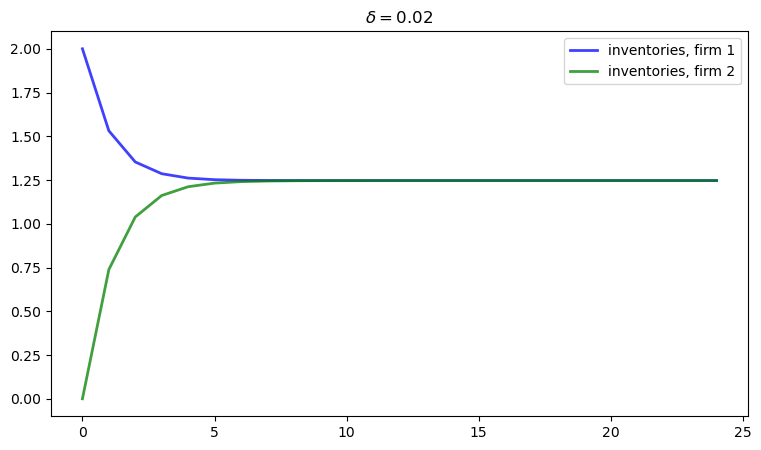
The first figure shows the dynamics of inventories for each firm when the parameters are
δ = 0.02
D = np.array([[-1, 0.5], [0.5, -1]])
b = np.array([25, 25])
c1 = c2 = np.array([1, -2, 1])
e1 = e2 = np.array([10, 10, 3])
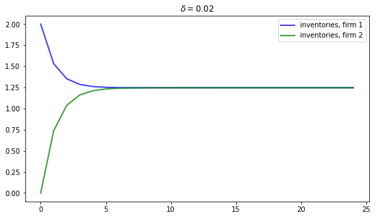
Inventories trend to a common steady state.
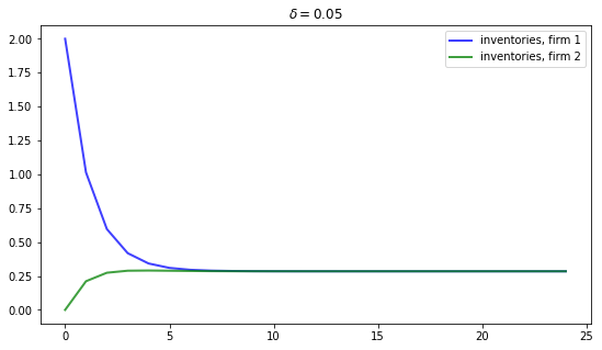
If we increase the depreciation rate to \(\delta = 0.05\), then we expect steady state inventories to fall.
This is indeed the case, as the next figure shows
In this exercise, reproduce the figure when \(\delta = 0.02\).
Solution
We treat the case \(\delta = 0.02\)
δ = 0.02
D = np.array([[-1, 0.5], [0.5, -1]])
b = np.array([25, 25])
c1 = c2 = np.array([1, -2, 1])
e1 = e2 = np.array([10, 10, 3])

δ_1 = 1 - δ
Recalling that the control and state are
we set up the matrices as follows:
# ==  Create matrices needed to compute the Nash feedback equilibrium == #

A = np.array([[δ_1,      0,    -δ_1 * b[0]],
              [  0,    δ_1,    -δ_1 * b[1]],
              [  0,      0,             1]])

B1 = δ_1 * np.array([[1, -D[0, 0]],
                     [0, -D[1, 0]],
                     [0,       0]])
B2 = δ_1 * np.array([[0, -D[0, 1]],
                     [1, -D[1, 1]],
                     [0,       0]])

R1 = -np.array([[0.5 * c1[2],     0,    0.5 * c1[1]],
                [          0,     0,              0],
                [0.5 * c1[1],     0,         c1[0]]])
R2 = -np.array([[0,               0,              0],
                [0,     0.5 * c2[2],    0.5 * c2[1]],
                [0,     0.5 * c2[1],         c2[0]]])

Q1 = np.array([[-0.5 * e1[2], 0], [0, D[0, 0]]])
Q2 = np.array([[-0.5 * e2[2], 0], [0, D[1, 1]]])

S1 = np.zeros((2, 2))
S2 = np.copy(S1)

W1 = np.array([[           0,             0],
               [           0,             0],
               [-0.5 * e1[1],    b[0] / 2.]])
W2 = np.array([[           0,             0],
               [           0,             0],
               [-0.5 * e2[1],    b[1] / 2.]])

M1 = np.array([[0, 0], [0, D[0, 1] / 2.]])
M2 = np.copy(M1)
We can now compute the equilibrium using qe.nnash
F1, F2, P1, P2 = qe.nnash(A, B1, B2, R1,
                          R2, Q1, Q2, S1,
                          S2, W1, W2, M1, M2)

print("\nFirm 1's feedback rule:\n")
print(F1)

print("\nFirm 2's feedback rule:\n")
print(F2)
Firm 1's feedback rule:

[[ 2.43666582e-01  2.72360627e-02 -6.82788293e+00]
 [ 3.92370734e-01  1.39696451e-01 -3.77341073e+01]]

Firm 2's feedback rule:

[[ 2.72360627e-02  2.43666582e-01 -6.82788293e+00]
 [ 1.39696451e-01  3.92370734e-01 -3.77341073e+01]]
Now let’s look at the dynamics of inventories, and reproduce the graph corresponding to \(\delta = 0.02\)
AF = A - B1 @ F1 - B2 @ F2
n = 25
x = np.empty((3, n))
x[:, 0] = 2, 0, 1
for t in range(n-1):
    x[:, t+1] = AF @ x[:, t]
I1 = x[0, :]
I2 = x[1, :]
fig, ax = plt.subplots(figsize=(9, 5))
ax.plot(I1, 'b-', lw=2, alpha=0.75, label='inventories, firm 1')
ax.plot(I2, 'g-', lw=2, alpha=0.75, label='inventories, firm 2')
ax.set_title(rf'$\delta = {δ}$')
ax.legend()
plt.show()