56. Cake Eating VI: EGM with JAX#
56.1. Overview#
In this lecture, we’ll implement the endogenous grid method (EGM) using JAX.
This lecture builds on Cake Eating V: The Endogenous Grid Method, which introduced EGM using NumPy.
By converting to JAX, we can leverage fast linear algebra, hardware accelerators, and JIT compilation for improved performance.
We’ll also use JAX’s vmap function to fully vectorize the Coleman-Reffett operator.
Let’s start with some standard imports:
import matplotlib.pyplot as plt
import jax
import jax.numpy as jnp
import quantecon as qe
from typing import NamedTuple
56.2. Implementation#
For details on the savings problem and the endogenous grid method (EGM), please see Cake Eating V: The Endogenous Grid Method.
Here we focus on the JAX implementation of EGM.
We use the same setting as in Cake Eating V: The Endogenous Grid Method:
\(u(c) = \ln c\),
production is Cobb-Douglas, and
the shocks are lognormal.
Here are the analytical solutions for comparison.
def v_star(x, α, β, μ):
    """
    True value function
    """
    c1 = jnp.log(1 - α * β) / (1 - β)
    c2 = (μ + α * jnp.log(α * β)) / (1 - α)
    c3 = 1 / (1 - β)
    c4 = 1 / (1 - α * β)
    return c1 + c2 * (c3 - c4) + c4 * jnp.log(x)

def σ_star(x, α, β):
    """
    True optimal policy
    """
    return (1 - α * β) * x
The Model class stores only the data (grids, shocks, and parameters).
Utility and production functions will be defined globally to work with JAX’s JIT compiler.
class Model(NamedTuple):
    β: float              # discount factor
    μ: float              # shock location parameter
    s: float              # shock scale parameter
    grid: jnp.ndarray     # state grid
    shocks: jnp.ndarray   # shock draws
    α: float              # production function parameter


def create_model(β: float = 0.96,
                 μ: float = 0.0,
                 s: float = 0.1,
                 grid_max: float = 4.0,
                 grid_size: int = 120,
                 shock_size: int = 250,
                 seed: int = 1234,
                 α: float = 0.4) -> Model:
    """
    Creates an instance of the cake eating model.
    """
    # Set up grid
    grid = jnp.linspace(1e-4, grid_max, grid_size)

    # Store shocks (with a seed, so results are reproducible)
    key = jax.random.PRNGKey(seed)
    shocks = jnp.exp(μ + s * jax.random.normal(key, shape=(shock_size,)))

    return Model(β=β, μ=μ, s=s, grid=grid, shocks=shocks, α=α)
Here’s the Coleman-Reffett operator using EGM.
The key JAX feature here is vmap, which vectorizes the computation over the grid points.
def K(σ_array: jnp.ndarray, model: Model) -> jnp.ndarray:
    """
    The Coleman-Reffett operator using EGM

    """

    # Simplify names
    β, α = model.β, model.α
    grid, shocks = model.grid, model.shocks

    # Determine endogenous grid
    x = grid + σ_array  # x_i = k_i + c_i

    # Linear interpolation of policy using endogenous grid
    σ = lambda x_val: jnp.interp(x_val, x, σ_array)

    # Define function to compute consumption at a single grid point
    def compute_c(k):
        vals = u_prime(σ(f(k, α) * shocks)) * f_prime(k, α) * shocks
        return u_prime_inv(β * jnp.mean(vals))

    # Vectorize over grid using vmap
    compute_c_vectorized = jax.vmap(compute_c)
    c = compute_c_vectorized(grid)

    return c
We define utility and production functions globally.
Note that f and f_prime take α as an explicit argument, allowing them to work with JAX’s functional programming model.
# Define utility and production functions with derivatives
u = lambda c: jnp.log(c)
u_prime = lambda c: 1 / c
u_prime_inv = lambda x: 1 / x
f = lambda k, α: k**α
f_prime = lambda k, α: α * k**(α - 1)
Now we create a model instance.
α = 0.4

model = create_model(α=α)
grid = model.grid
The solver uses JAX’s jax.lax.while_loop for the iteration and is JIT-compiled for speed.
@jax.jit
def solve_model_time_iter(model: Model,
                          σ_init: jnp.ndarray,
                          tol: float = 1e-5,
                          max_iter: int = 1000) -> jnp.ndarray:
    """
    Solve the model using time iteration with EGM.
    """

    def condition(loop_state):
        i, σ, error = loop_state
        return (error > tol) & (i < max_iter)

    def body(loop_state):
        i, σ, error = loop_state
        σ_new = K(σ, model)
        error = jnp.max(jnp.abs(σ_new - σ))
        return i + 1, σ_new, error

    # Initialize loop state
    initial_state = (0, σ_init, tol + 1)

    # Run the loop
    i, σ, error = jax.lax.while_loop(condition, body, initial_state)

    return σ
We solve the model starting from an initial guess.
σ_init = jnp.copy(grid)
σ = solve_model_time_iter(model, σ_init)
Let’s plot the resulting policy against the analytical solution.
x = grid + σ  # x_i = k_i + c_i

fig, ax = plt.subplots()

ax.plot(x, σ, lw=2,
        alpha=0.8, label='approximate policy function')

ax.plot(x, σ_star(x, model.α, model.β), 'k--',
        lw=2, alpha=0.8, label='true policy function')

ax.legend()
plt.show()
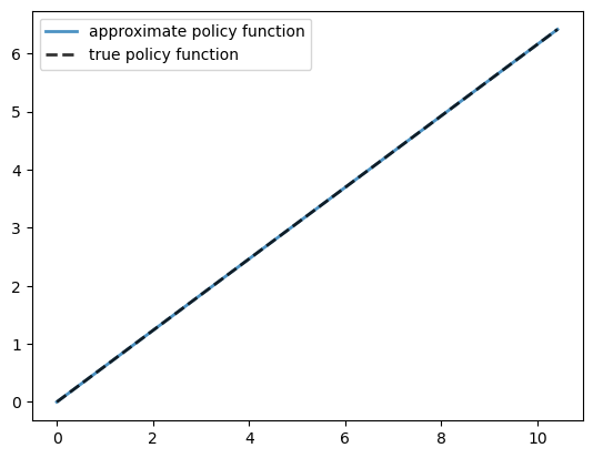
The fit is very good.
max_dev = jnp.max(jnp.abs(σ - σ_star(x, model.α, model.β)))
print(f"Maximum absolute deviation: {max_dev:.7}")
Maximum absolute deviation: 1.430511e-06
The JAX implementation is very fast thanks to JIT compilation and vectorization.
with qe.Timer(precision=8):
    σ = solve_model_time_iter(model, σ_init).block_until_ready()
0.00272655 seconds elapsed
This speed comes from:
JIT compilation of the entire solver
Vectorization via
vmapin the Coleman-Reffett operatorUse of
jax.lax.while_loopinstead of a Python loopEfficient JAX array operations throughout
56.3. Exercises#
Exercise 56.1
Solve the stochastic cake eating problem with CRRA utility
Compare the optimal policies for values of \(\gamma\) approaching 1 from above (e.g., 1.05, 1.1, 1.2).
Show that as \(\gamma \to 1\), the optimal policy converges to the policy obtained with log utility (\(\gamma = 1\)).
Hint: Use values of \(\gamma\) close to 1 to ensure the endogenous grids have similar coverage and make visual comparison easier.
Solution
We need to create a version of the Coleman-Reffett operator and solver that work with CRRA utility.
The key is to parameterize the utility functions by \(\gamma\).
def u_crra(c, γ):
    return (c**(1 - γ) - 1) / (1 - γ)

def u_prime_crra(c, γ):
    return c**(-γ)

def u_prime_inv_crra(x, γ):
    return x**(-1/γ)
Now we create a version of the Coleman-Reffett operator that takes \(\gamma\) as a parameter.
def K_crra(σ_array: jnp.ndarray, model: Model, γ: float) -> jnp.ndarray:
    """
    The Coleman-Reffett operator using EGM with CRRA utility
    """
    # Simplify names
    β, α = model.β, model.α
    grid, shocks = model.grid, model.shocks

    # Determine endogenous grid
    x = grid + σ_array

    # Linear interpolation of policy using endogenous grid
    σ = lambda x_val: jnp.interp(x_val, x, σ_array)

    # Define function to compute consumption at a single grid point
    def compute_c(k):
        vals = u_prime_crra(σ(f(k, α) * shocks), γ) * f_prime(k, α) * shocks
        return u_prime_inv_crra(β * jnp.mean(vals), γ)

    # Vectorize over grid using vmap
    compute_c_vectorized = jax.vmap(compute_c)
    c = compute_c_vectorized(grid)

    return c
We also need a solver that uses this operator.
@jax.jit
def solve_model_crra(model: Model,
                     σ_init: jnp.ndarray,
                     γ: float,
                     tol: float = 1e-5,
                     max_iter: int = 1000) -> jnp.ndarray:
    """
    Solve the model using time iteration with EGM and CRRA utility.
    """

    def condition(loop_state):
        i, σ, error = loop_state
        return (error > tol) & (i < max_iter)

    def body(loop_state):
        i, σ, error = loop_state
        σ_new = K_crra(σ, model, γ)
        error = jnp.max(jnp.abs(σ_new - σ))
        return i + 1, σ_new, error

    # Initialize loop state
    initial_state = (0, σ_init, tol + 1)

    # Run the loop
    i, σ, error = jax.lax.while_loop(condition, body, initial_state)

    return σ
Now we solve for \(\gamma = 1\) (log utility) and values approaching 1 from above.
γ_values = [1.0, 1.05, 1.1, 1.2]
policies = {}

model_crra = create_model(α=α)

for γ in γ_values:
    σ_init = jnp.copy(model_crra.grid)
    σ_gamma = solve_model_crra(model_crra, σ_init, γ).block_until_ready()
    policies[γ] = σ_gamma
    print(f"Solved for γ = {γ}")
Solved for γ = 1.0
Solved for γ = 1.05
Solved for γ = 1.1
Solved for γ = 1.2
Plot the policies on their endogenous grids.
fig, ax = plt.subplots()

for γ in γ_values:
    x = model_crra.grid + policies[γ]
    if γ == 1.0:
        ax.plot(x, policies[γ], 'k-', linewidth=2,
                label=f'γ = {γ:.2f} (log utility)', alpha=0.8)
    else:
        ax.plot(x, policies[γ], label=f'γ = {γ:.2f}', alpha=0.8)

ax.set_xlabel('State x')
ax.set_ylabel('Consumption σ(x)')
ax.legend()
ax.set_title('Optimal policies: CRRA utility approaching log case')
plt.show()
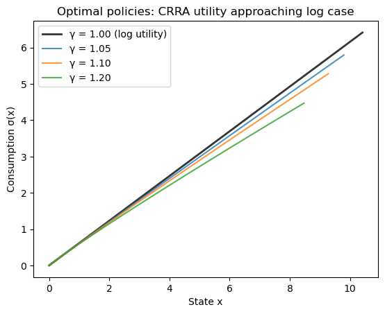
Note that the plots for \(\gamma > 1\) do not cover the entire x-axis range shown.
This is because the endogenous grid \(x = k + \sigma(k)\) depends on the consumption policy, which varies with \(\gamma\).
Let’s check the maximum deviation between the log utility case (\(\gamma = 1.0\)) and values approaching from above.
for γ in [1.05, 1.1, 1.2]:
    max_diff = jnp.max(jnp.abs(policies[1.0] - policies[γ]))
    print(f"Max difference between γ=1.0 and γ={γ}: {max_diff:.6}")
Max difference between γ=1.0 and γ=1.05: 0.619199
Max difference between γ=1.0 and γ=1.1: 1.1362
Max difference between γ=1.0 and γ=1.2: 1.94592
As expected, the differences decrease as \(\gamma\) approaches 1 from above, confirming convergence.